4. User Manual¶

4.1. Thermal Processing¶

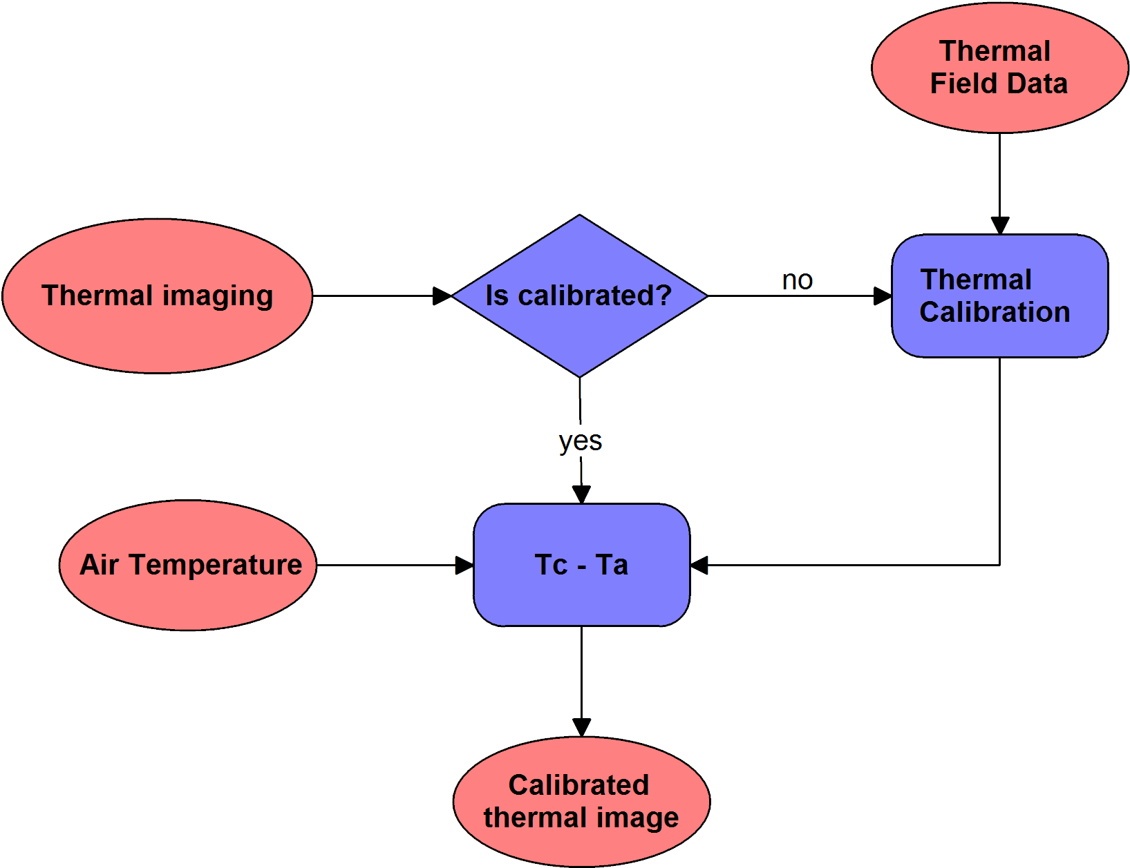
4.1.1. Thermal Calibration¶

This module allows to calibrate thermal images based on the calibration data obtained in the field. During the calibration process, spectral data is linearly correlated with selected field reflectance spectral.

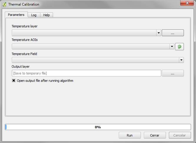
4.1.1.1. Required Input Parameters¶

Temperature layer: Thermal raster
Temperature AOIs: Shapefile containing information on temperature field measurements
Temperature Field: Vector’s field containing temperature

4.1.1.2. Output Parameters¶

Output layer: Calibrated thermal raster output.

4.1.2. Tc - Ta¶

This module normalizes the temperature raster image according to the air temperature during the image acquisition.

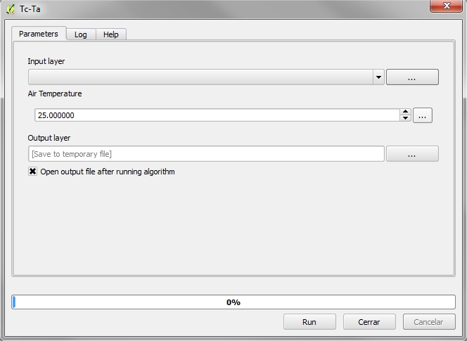
4.1.2.1. Required Input Parameters¶

Input layer: Thermal raster
Air temperature: Constant air temperature measure at flight time

4.1.2.2. Output Parameters¶

Output layer: Thermal raster output including normalized temperature.

4.2. LiDAR Processing¶

LiDAR data is often provided as a number of tiles or flight lines. Depending on computers capacity, in some cases it might be convenient to merge flight files into a single file, or to divide data in overlapping tiles with an appropriate size.

Due to ThermoLiDAR software uses SPDLib suite for LiDAR data manipulation, data has to be converted into the native SPDLib file format. This means that LiDAR data must be converted into Sorted Pulse Data format (SPD) from LAS files, which is the file standard for the interchange of LASer data recommended by the American Society for Photogrammetry and Remote Sensing (ASPRS). Noisy data can be eventually removed before being processed. Once the SPD files have been obtained, ground points are classified and then point heights relative to the ground are inferred. Ground and no-ground points are interpolated to generate DTM, DSM and CHM. From height information a range of metrics mainly applied to forestry applications -but not only- can be derived. Here below this workflow is depicted.

LiDAR workflow using the SPDLib toolset. In this case, SPD format files are supplied as input. Names of SPDLib commands are highlighted in bold font (i.e. spdmerge, spdtranslate, spddeftiles, etc.). Pink boxes represent output products. [Bunting2013]

4.2.1. Convert between formats¶

Since LiDAR processing modules make use of SPDLib tools, the first step is to convert the input dataset into SPD files. There are two types of SPD files, non-indexed and indexed. A format translation module has been included in QGIS to this purpose. The module allows the conversion between different formats and it is also used to re-project data.

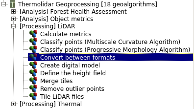
The module for format convertion is located in the LiDAR submenu of the ThermoLiDAR Toolbox

4.2.1.1. Supported file formats¶

ThermoLiDAR plugin supports SPD/UPD, LAS and a wide range of ASCII formats but the current level of support is not intended to encompass all the available formats.

4.2.1.1.1. SPD/UPD¶

The Sorted Pulse Data (SPD) file format (Bunting, 2013) has been designed specifically for the storage of LiDAR waveform and discrete return data acquired by TLS, ALS and space borne systems, and includes support for multiple wavelengths within a single file. The SPD format also supports 2D spatial indexing of the pulses, and the Unsorted Pulse Data (UPD) files are SPD files without a spatial index.

4.2.1.1.2. LAS¶

The LASer (LAS) file format supported is aligned with the LAS v1.2 specifications. LAS 1.2 files are exported through the LibLAS library so as with the importer only discrete return data are supported.

4.2.1.1.3. ASCII¶

The ASCII format requires a schema written in XML to be supplied. The parse expects a single return per line and the resulting pulses will only contain a single return. The following are some examples of schemas for common ASCII formats.

A schema for the PTS format:

<?xml version="1.0" encoding="UTF-8" ?>
<line delimiter=" " comment="#" ignorelines="0" >
   <field name="X" type="spd_double" index="0" />
   <field name="Y" type="spd_double" index="1" />
   <field name="Z" type="spd_float" index="2" />
   <field name="AMPLITUDE_RETURN" type="spd_uint" index="3" />
   <field name="RED" type="spd_uint" index="4" />
   <field name="GREEN" type="spd_uint" index="5" />
   <field name="BLUE" type="spd_uint" index="6" />
</line>

A schema for the XYZ format:

<?xml version="1.0" encoding="UTF-8" ?>
<line delimiter="," comment="#" ignorelines="0" >
   <field name="X" type="spd_double" index="0" />
   <field name="Y" type="spd_double" index="1" />
   <field name="Z" type="spd_float" index="2" />
   <field name="AMPLITUDE_RETURN" type="spd_uint" index="3" />
</line>

4.2.1.2. Reprojection¶

It is possible to define the projection of the SPD file explicitly using the input and output projection. Both options expect a text file containing the WKT (Well Known Text) string representing the projection information. In order to change projection, the input projection option is not required, but if it is known, then it should be advantageous to provide it.

4.2.1.3. Memory Requirements¶

When converting to an UPD very little memory is required as only a few pulses are held in memory at any one time, this is because no sorting of the pulses is required. On the other hand when generating an SPD file the data needs to be spatially sorted. Therefore, the whole file is read into memory and sorted into the spatial grid before being written output the file. This requires enough memory to store the whole dataset and index data structure in memory. If memory is not sufficient to complete this operation the file needs to be split into blocks to fit into memory.

The option to select splitting the file to disk while building the SPD file is temporal path which is the path and base file name while the tiles will be written. The num rows parameter specifies the number of rows of the final SPD file that will be written to each temporary tile. Note that the tile height in is binsize x num rows (in units the data is projected). The num columns option maybe set where datasets are very wide such that the tiles are not the full width of the output file. Whether this option is used, the final SPD file will result in a non-sequential rather than a sequential file. This means the data on disk is not order left-to-right top-to-bottom or top-left to bottom-right, which has some performance benefits. Obviously, allowing the SPD file to be built in stages is slower but once completed it is faster to make spatial queries within the file. Besides, other processing steps (i.e., classification and interpolations) can be applied to the whole file with only relatively small memory requirements.

4.2.1.4. Parameters¶

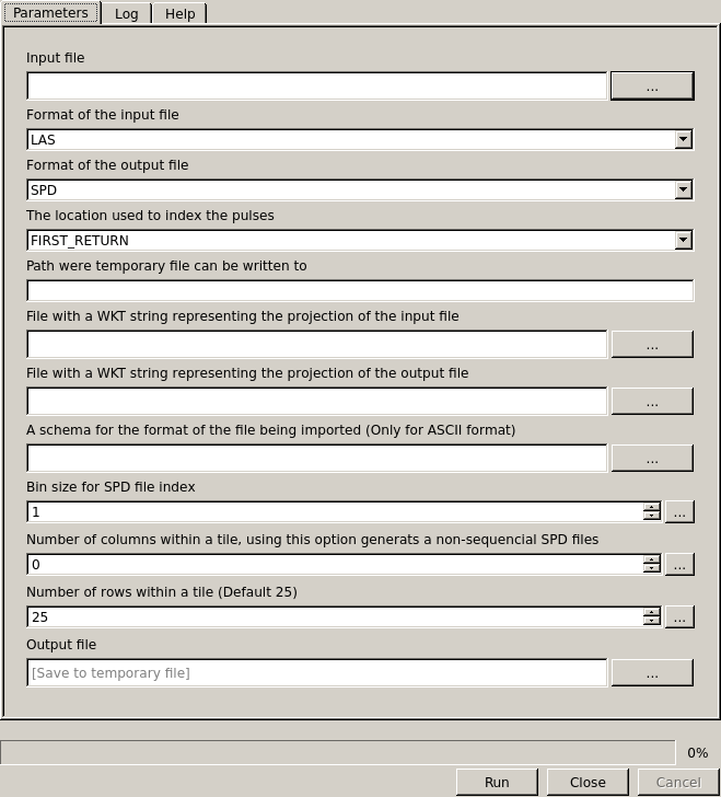
Interface to convert between different data formats

4.2.1.4.1. Required Input Parameters¶

Input: SPD file that contains the LiDAR point clouds.
Index: The location used to index the pulses and points (required):
- FIRST_RETURN
- LAST_RETURN
Input Format: Format of the input file (Default SPD).
- SPD: SPD input format with or without spatial index
- ASCII: ASCII input format
- LAS/LAZ: Both zipped or normal LAS input format
- LASNP: LAS input without pulse information
Ouput Format: Format of the output file (Default SPD).
- SPD: SPD output format
- UPD: SPD output format without spatial index
- ASCII: ASCII output format
- LAS: LAS output format
- LAZ: Zipped LAS output format

4.2.1.4.2. Optional Input Parameters¶

Binsize: (float) Bin size for SPD file index (Default 1)
Schema: (string) schema for the format of the ASCII file being imported
Input Projection: (string) WKT string representing the projection of the input file
Output Projection: (string) WKT string representing the projection of the output file
Num. Columns: (integer) Number of columns within a block (Default 0) - Note values greater than 1 result in a non-sequential SPD file.
Num. Rows: (integer) Number of rows within a block (Default 25)
Temporal Path: (string) Path where temporary files can be written to.

4.2.1.4.3. Output Parameters¶

Output: The output SPD file

4.2.2. Merge files¶

In some situations it might be convenient to merge various files into a single SPD file. The merging module merges compatible files into a single non-indexed SPD file. It is possible to provide the projection information of the output file and input files if known.

This module allows displaying classes and returns IDs of the input files with list returns IDs and list classes options, respectively. The ignore checks option forces the input files to be merged in case files come from different sources or have different bin sizes.

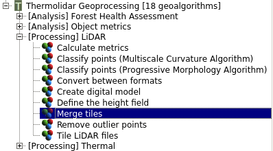
The module for merging files is located in the LiDAR submenu of the ThermoLiDAR toolbox

4.2.2.1. Parameters¶

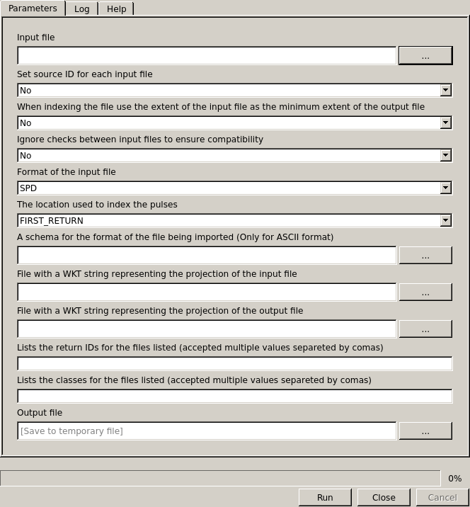
Interface to merge compatible files into a single non-indexed SPD file

4.2.2.1.1. Required Input Parameters¶

Input: SPD file that contains the LiDAR point clouds (accept multiple files separated by comas).
Index: The location used to index the pulses and points (required):
- FIRST_RETURN
- LAST_RETURN
Input Format: Format of the input file (Default SPD).
- SPD: SPD input format with or without spatial index
- ASCII: ASCII input format
- LAS/LAZ: Both zipped or normal LAS input format
- LASNP: LAS input without pulse information

4.2.2.1.2. Optional Input Parameters¶

List Returns IDs: (list of files) Lists the return IDs for the files listed (accept multiple files separated by comas).
List Classes: (list of files) Lists the classes for the files listed (accept multiple files separated by comas).
Keep Extent: (Yes/No) Use the extent of the input files as the minimum extent of the output file when indexing the file.
Source ID: (Yes/No) Set source ID for each input file
Ignore Checks: (Yes/No) Ignore checks between input files to ensure compatibility
Schema: (string) schema for the format of the ASCII file being imported
Input Projection: (string) WKT string representing the projection of the input file
Output Projection: (string) WKT string representing the projection of the output file

4.2.2.1.3. Output Parameters¶

Output: The output SPD file

4.2.3. Split data into tiles¶

LiDAR data is supplied as flight lines or tiles with different shapes and sizes. It is always useful to divide laser data into equally sized square tiles, though. This helps to store, manage and access data easily. Single tiles should meet memory requirements in order to reduce computational times, which determines the maximum size of each file given an average point density. Overlapping zones between tiles help to prevent border errors and guarantee continuous raster models.

ThermoLiDAR has a built-in tool to create tiles given tiles size and the overlap. Output tiles are saved into the output path (this includes path and prefix) and are named as _rowYYcolXX.spd, being YY and XX the number of row and column of the corresponding tile. Tiles definition is stored in an output XML file (output xml) containing their column, row, extent and core extent (tile extent without overlap).

<tiles columns="23" overlap="50" rows="16" xmax="256500" xmin="239343.510" xtilesize="750" ymax="707224.300" ymin="695246.440" ytilesize="750">
   <tile col="1" corexmax="240093.510" corexmin="239343.510" coreymax="695996.440" coreymin="695246.440" file="" row="1" xmax="240143.510" xmin="239293.510" ymax="696046.440" ymin="695196.440"/>
   <tile col="2" corexmax="240843.510" corexmin="240093.510" coreymax="695996.440" coreymin="695246.440" file="" row="1" xmax="240893.510" xmin="240043.510" ymax="696046.440" ymin="695196.440"/>

   ...

   <tile col="22" corexmax="255843.510" corexmin="255093.510" coreymax="707246.440" coreymin="706496.440" file="" row="16" xmax="255893.510" xmin="255043.510" ymax="707296.440" ymin="706446.440"/>
   <tile col="23" corexmax="256593.510" corexmin="255843.510" coreymax="707246.440" coreymin="706496.440" file="" row="16" xmax="256643.510" xmin="255793.510" ymax="707296.440" ymin="706446.440"/>
</tiles>

The module supports to create single tiles (SINGLE option) by supplying row and column, or to generate the complete set of tiles (ALL option).

The module also creates an auxiliary file listing the input LiDAR which can be eventually kept (keep file list) once the module has finished. It might happen that some tiles are empty; in that case those files can be removed enabling the delete tiles option.

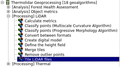
The module for tiling LiDAR data is within the LiDAR submenu of the ThermoLiDAR toolbox

4.2.3.1. Parameters¶

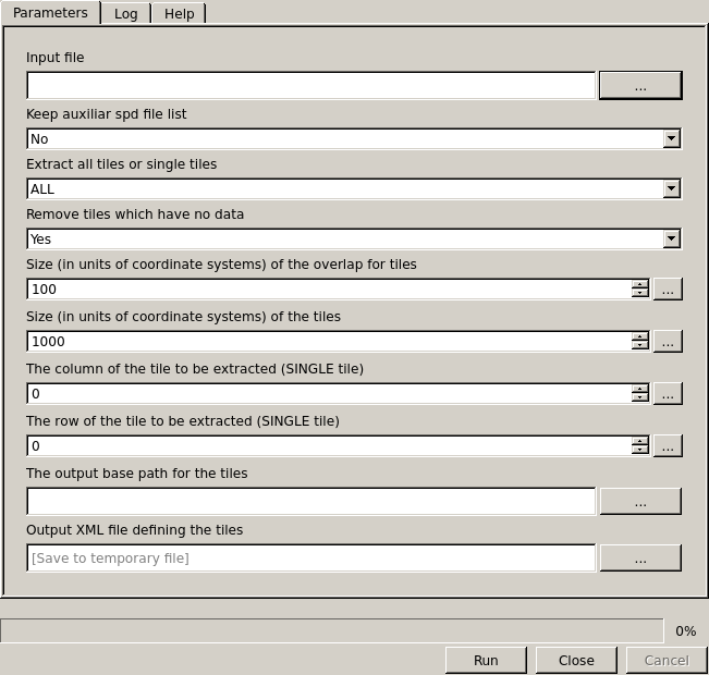
Interface for tiling a set of SPD files

4.2.3.1.1. Required Input Parameters¶

Input: SPD file that contains the LiDAR point clouds (accept multiple files separated by comas).

4.2.3.1.2. Optional Input Parameters¶

Extract Tiles: Where to extract
- ALL: Create all tiles
- SINGLE: Extract an individual tile given its row and column
Delete Tiles: (Yes/No) If shapefile exists delete it and then run
Keep File List: (Yes/No) Keep auxiliary file containing a list of the input files to be tiled
Tile Size: (float) Size (in units of the coordinate system) of the square tiles (Default: 1000)
Overlap Size: (float) Size (in units of coordinate systems) of the overlap for tiles (Default 100)
Column: (integer) The column of the tile to be extracted (only with single)
Row: (integer) The row of the tile to be extracted (only with single)
Output Path: (string) The output XML file that contains the tiles definition

4.2.3.1.3. Output Parameters¶

Output XML: The output XML file that contains the tiles definition

4.2.4. Remove Noise¶

Many factors may introduce errors in LiDAR point clouds, including water vapour clouds, multipath, poor equipment calibration, or even a flock of birds. In order to avoid further errors and artefacts in final digital models and poor assess of height metrics, those points have to be removed.

This module removes vertical noise from LiDAR datasets by means of three different. Upper and lower absolute thresholds will clip the file to fit these values. Relative threshold will remove, for each bin within a SPD file, points outside the upper and lower values relative to the median height. Whilst global threshold will use the whole SPD file to calculate the median height and remove points relative to it.

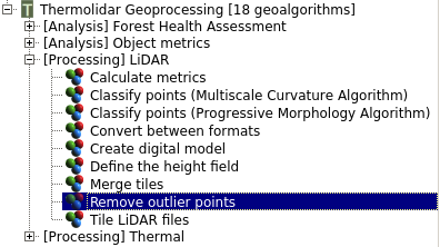
The module for removing noise from data is located in the LiDAR submenu of the ThermoLiDAR toolbox

4.2.4.1. Parameters¶

Interface for tiling a set of SPD files

4.2.4.1.1. Required Input Parameters¶

Input: SPD file that contains the LiDAR point clouds.

4.2.4.1.2. Optional Input Parameters¶

Global Rel. Upper Threshold: (float) Global relative to median upper threshold for returns which are to be removed
Global Rel. Lower Threshold: (float) Global relative to median lower threshold for returns which are to be removed
Relative Upper Threshold: (float) Relative to median upper threshold for returns which are to be removed
Relative Lower Threshold: (float) Relative to median lower threshold for returns which are to be removed
Absolute Upper Threshold: (float) Absolute upper threshold for returns which are to be removed
Absolute Lower Threshold: (float) Absolute lower threshold for returns which are to be removed
Column: (integer) The column of the tile to be extracted (only with single)
Row: (integer) The row of the tile to be extracted (only with single)

4.2.4.1.3. Output Parameters¶

Output: The output SPD file without noise

4.2.5. Classify Ground Returns¶

Two different classification algorithms have been implemented into the plugin. These algorithms also called filters allow the classification of the LiDAR points, identifying which point belong to the ground. The filters implement the Progressive Morphology (Zhang et al., 2003; [Zhang2003]) and the Multiscale Curvature (Evans and Hudak, 2007; [EvansHudak2007]) methodologies.

4.2.5.1. Progressive Morphology filter¶

To classify ground returns an implementation of the Progressive Morphology algorithm (PMF) has been provided. The algorithm QGIS interface has only three options to be set. Under most circumstances the default parameters will be fit the purpose and it is recommended to use the simplest parameters configuration given by default.

The class option allows to apply the filter to particular classes (i.e., if ground returns have been already classified but they need tidying up).

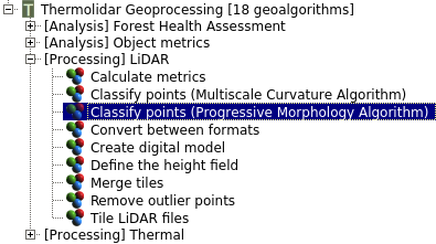
The module that implements the PMF algorithm to classify ground is within the LiDAR submenu of the ThermoLiDAR toolbox

4.2.5.1.1. Parameters¶

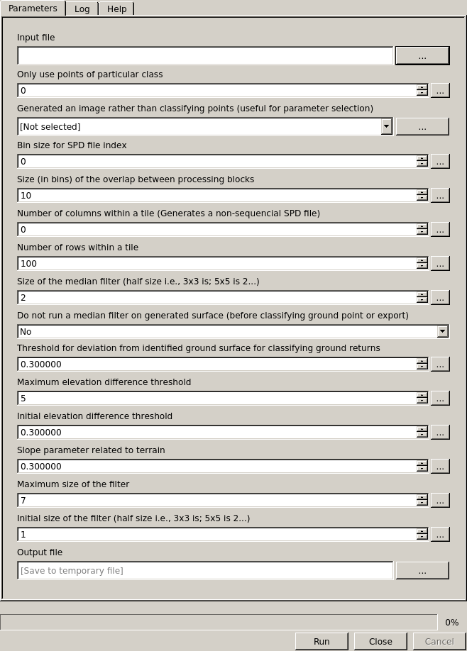
Interface of the Progressive Morphology Algorithm to classify ground points

4.2.5.1.1.1. Required Input Parameters¶

Input: SPD file that contains the LiDAR point clouds.

4.2.5.1.1.2. Optional Input Parameters¶

Binsize: (float) Bin size for SPD file index (Default 1)
Class: (integer) Only use points of particular class
Ground Threshold: (float) Threshold for deviation from identified ground surface for classifying the ground returns (Default 0.3)
Median Filter: (integer) Size of the median filter (half size i.e., 3x3 is 1) (Default 2)
No Median: (Yes/No) Do not run a median filter on generated surface
Max. Elevation: (float) Maximum elevation difference threshold (Default 5)
Initial Elevation: (float) Initial elevation difference threshold (Default 0.3)
Slope: (float) Slope parameter related to terrain (Default 0.3)
Max. Filter: (float) Maximum size of the filter (Default 7)
Initial Filter: (float) Initial size of the filter (half size i.e., 3x3 is 1) (Default 1)
Overlap: (integer) Size (in bins) of the overlap between processing blocks (Default 10)
Num. Columns: (integer) Number of columns within a block (Default 0) - Note values greater than 1 result in a non-sequential SPD file.
Num. Rows: (integer) Number of rows within a block (Default 25)

4.2.5.1.1.3. Output Parameters¶

Output: The output SPD file containing classification

4.2.5.2. Multiscale Curvature filter¶

The plugins integrates an implementation of the Multiscale Curvature algorithm (MCC). As before, the QGIS interface has only three options to be set: input, output and class argument. Under most circumstances default parameters for the algorithm will be fit for purpose, but be careful that the bin size used within SPD is not too large as the processing will be at this resolution.

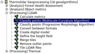
The module that implements the MCC algorithm to classify ground is within the LiDAR submenu of the ThermoLiDAR toolbox

4.2.5.2.1. Parameters¶

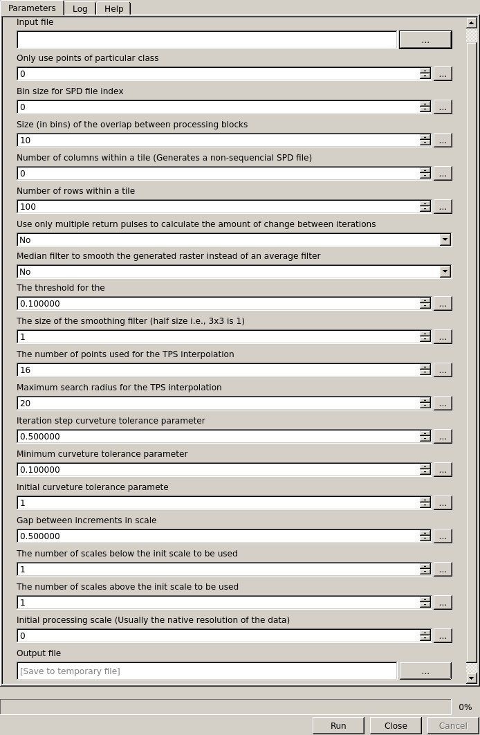
Interface of the Progressive Morphology Algorithm to classify ground points

4.2.5.2.1.1. Required Input Parameters¶

Input: SPD file that contains the LiDAR point clouds.

4.2.5.2.1.2. Optional Input Parameters¶

Binsize: (float) Bin size for SPD file index (Default 1)
Class: (integer) Only use points of particular class
Median: (Yes/No) Use a median filter to smooth the generated raster instead of a (mean) averaging filter.
Filter Size: (integer) The size of the smoothing filter (half size i.e., 3x3 is 1; Default = 1)
Num. Points Tps: (integer) The number of points used for the TPS interpolation (Default = 16)
Max. Radius Tps: (float) Maximum search radius for the TPS interpolation (Default = 20)
Step Curve Tolerance: (float) Iteration step curvature tolerance parameter (Default = 0.5)
Min. Curve Tolerance: (float) Minimum curvature tolerance parameter (Default = 0.1)
Initial Curve Tolerance: (float) Initial curvature tolerance parameter (Default = 1)
Scale Gaps: (float) Gap between increments in scale (Default = 0.5)
Num. Scales Below: (integer) The number of scales below the init scale to be used (Default = 1)
Num. Scales Above: (integer) The number of scales above the init scale to be used (Default = 1)
Initial Scale: (float) Initial processing scale, this is usually the native resolution of the data.
Max. Elevation Threshold: (float) Maximum elevation difference threshold (Default 5)
Initial Elevation Threshold: (float) Initial elevation difference threshold (Default 0.3)
Slope: (float) Slope parameter related to terrain (Default 0.3)
Max. Filter: (float) Maximum size of the filter (Default 7)
Initial Filter: (float) Initial size of the filter (half size i.e., 3x3 is 1) (Default 1)
Overlap: (integer) Size (in bins) of the overlap between processing blocks (Default 10)
Num. Columns: (integer) Number of columns within a block (Default 0) - Note values greater than 1 result in a non-sequential SPD file.
Num. Rows: (integer) Number of rows within a block (Default 25)

4.2.5.2.1.3. Output Parameters¶

Output: The output SPD file containing classification

4.2.5.3. Filter points depending on class¶

The class option applies the filter to returns of a particular class (i.e., ground returns). This represents a way to improve the ground return classification is to combine more than one filtering algorithm to take advantage of their particular strengths and weaknesses. In fact, a particularly useful combination is to first run the PMF algorithm where a thick slice is taken (e.g., 1 or 2 metres above the raster surface) and then the MCC is applied to find the ground returns (setting the class option to 3).

It can be also useful for TLS as it can take a thick slice with MCC algorithm and then use the PMF algorithm to tidy that result up to get a good overall ground classification.

4.2.6. Define Height field¶

SPD files supports both elevation corresponding to a vertical datum and an above-ground height for each discrete return. Before data can be used for generating a Canopy Height Model (CHM) or any height related metric, height field has to be populated. This can be done in two ways. The simplest way is to use a DTM of the same resolution as the SPD file bin size. The disadvantage of using a DTM is that it is if the DTM is not accurate it can introduce some artefacts. Using this method the only parameters are the input files, both LiDAR file and the DTM, and an output file. The raster DTM needs to the same resolution as the SPD grid and it can be any raster format supported by the GDAL library.

The other option is to interpolate a value for each point generating a continuous surface and reducing any artefacts. The recommended approach for the interpolation is to use the Natural Neighbour method, as demonstrated by Bater and Coops (2009; [BaterCoops2009]).

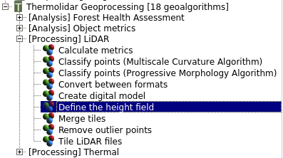
The module that defines the height above ground is located in the *LiDAR8 submenu of the ThermoLiDAR toolbox

4.2.6.1. Parameters¶

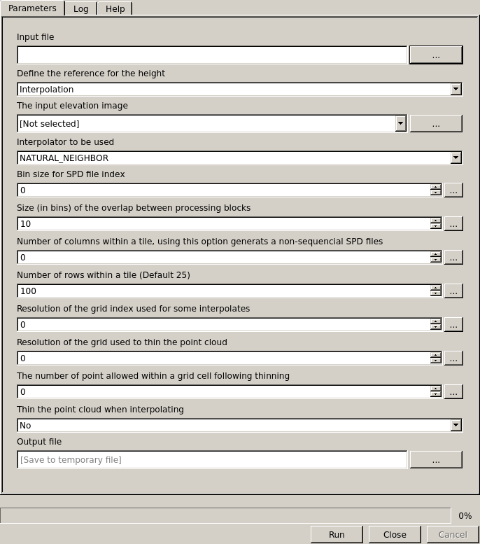
Interface of the module to define points heights from the ground

4.2.6.1.1. Required Input Parameters¶

Input: SPD file that contains the LiDAR point clouds.

4.2.6.1.2. Optional Input Parameters¶

Elevation: (raster) The input elevation image
Binsize: (float) Bin size for SPD file index (Default 1)
Interpolator: Different interpolation methods to choose from
- Natural Neighbor
- Nearest Neighbor
- TIN Plate
Thin: (Yes/No) Thin the point cloud when interpolating
Thin Resolution: (float) Resolution of the grid used to thin the point cloud
Point per Bin: (integer) The number of point allowed within a grid cell following thinning
Overlap: (integer) Size (in bins) of the overlap between processing blocks (Default 10)
Num. Columns: (integer) Number of columns within a block (Default 0) - Note values greater than 1 result in a non-sequential SPD file.
Num. Rows: (integer) Number of rows within a block (Default 25)

4.2.6.1.3. Output Parameters¶

Output: The output SPD file

4.2.7. Interpolation Module¶

The most common products that can be created from a LiDAR dataset are Digital Terrain Models (DTMs), Digital Surface Models (DSMs) and Canopy Height Models (CHMs). To produce those products, it is necessary to interpolate a raster surface from the classified ground returns and top surface points. Create Digital Model within the ThermoLiDAR plugin permits to generate these products by choosing model option.

A key parameter is the output raster resolution or binsize which needs to be a multiple of the SPD input file spatial index. Different interpolators can be selected with the interpolator option. This module supports many raster formats by means of the GDAL library.

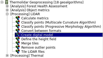
The interpolation module is in the LiDAR submenu of the ThermoLiDAR toolbox

4.2.7.1. Parameters¶

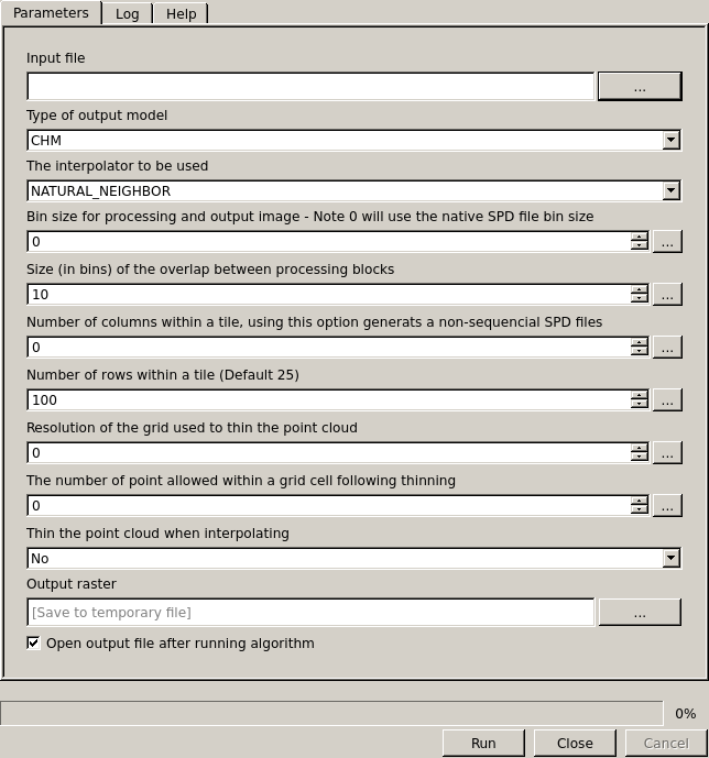
Interface to interpolate data

4.2.7.1.1. Required Input Parameters¶

Input: SPD file that contains the LiDAR point clouds.
MODEL:
- DTM: Digital Terrain Model
- MDS: Digital Surface Model
- CHM: Canopy Height Model

4.2.7.1.2. Optional Input Parameters¶

Binsize: (float) Bin size for SPD file index (Default 1)
Interpolator: Different interpolation methods to choose from
- Natural Neighbor
- Nearest Neighbor
- TIN Plate
Overlap: (integer) Size (in bins) of the overlap between processing blocks (Default 10)
Num. Columns: (integer) Number of columns within a block (Default 0) - Note values greater than 1 result in a non-sequential SPD file.
Num. Rows: (integer) Number of rows within a block (Default 25)

4.2.7.1.3. Output Parameters¶

Output: The raster file containing the interpolated model

4.2.7.2. Examples¶

Digital Surface Models (DSMs) are easily done by setting model to DSM. The module will perform an interpolation of the elevation information of all the points of the LiDAR file. The result is a surface representing the ground and all the objects attached to it as can be seen in figure below.

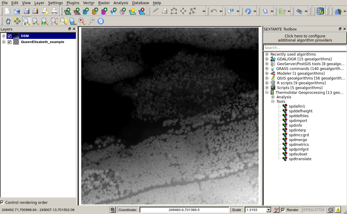
Example of visualization in grey scales of a DSM (1m resolution) generated with the ThermoLiDAR plugin

In case ground returns have been classified, then to interpolate elevation information of ground points will generate a Digital Terrain Model (DTM). For this purpose model has to be set to DTM. The output raster represents the bare ground surface (see next figure).

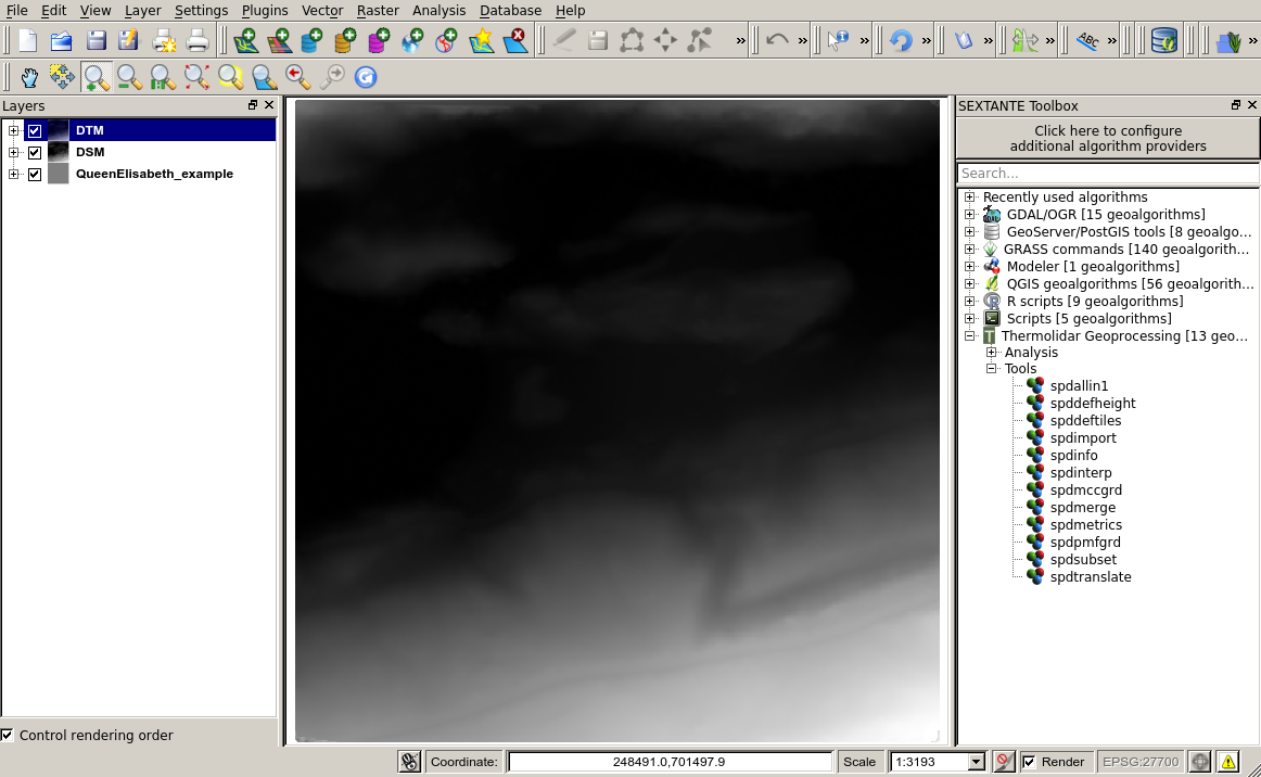
Example of visualization in grey scales of a DTM (1m resolution) generated with the ThermoLiDAR plugin

In a forest environment, those points not classified as ground are commonly classified as vegetation. To interpolate the height above ground information of vegetation points produces a Canopy Height Model (CHM). In this case, the model option is set to CHM. The result is raster where canopies are perfectly depicted and ground (see figure below).

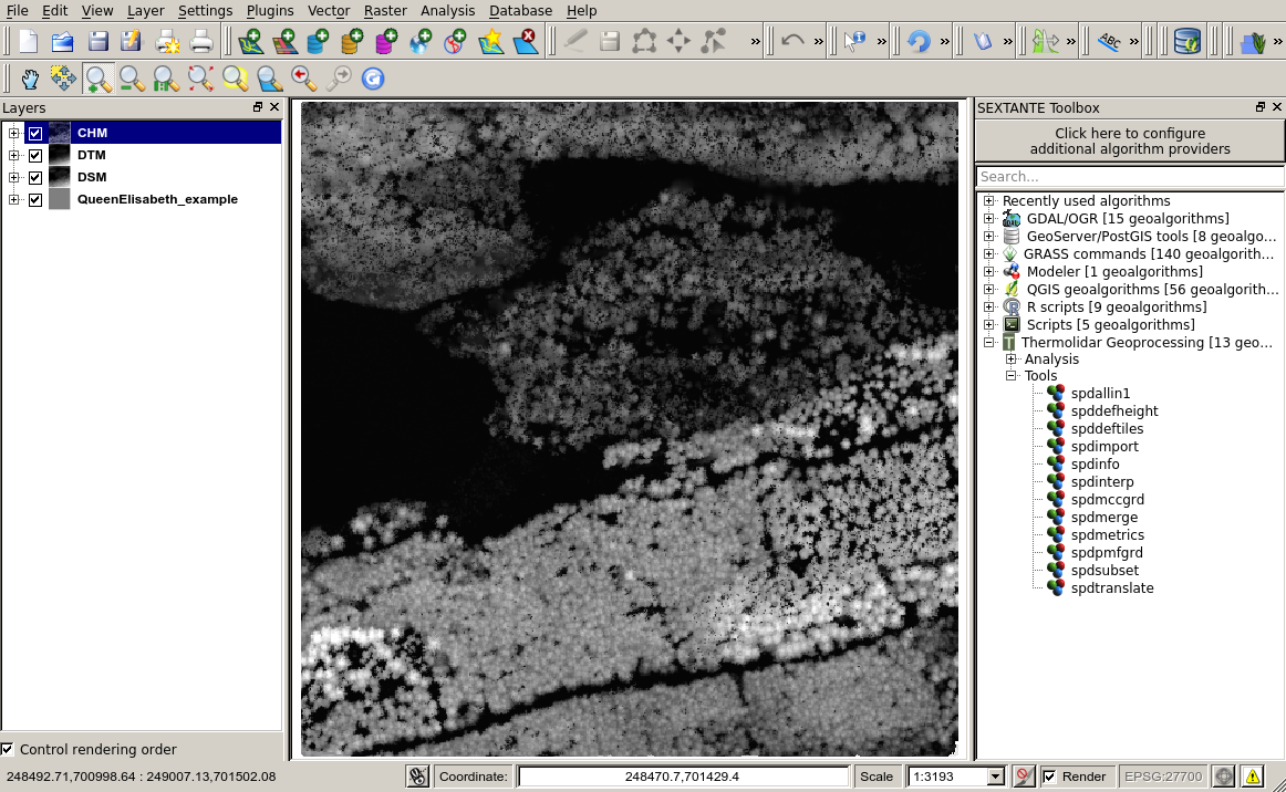
Example of visualization in grey scales of a CHM (1m resolution) generated with the ThermoLiDAR plugin

4.2.8. Generate metrics¶

ThermoLiDAR plugin is able to calculated different metrics at the same time if they are defined in an XML file. Metrics can be simple statistical moments, percentiles of point heights, or even count ratios. Mathematical operators can also be applied to either other metrics or operators, allowing a wider range of LiDAR metrics to be derived.

The XML file has to be defined a priori with a hierarchical list of metrics and operators. Within the metrics tags a list of metrics can be provided by the metric tag. Within each metric the field attribute is used to name the raster band or vector attribute.

The module supports different output data formats, that is, raster (all GDAL formats) and vector. Raster option extends the output to the entire input file, assessing the metrics for each pixel the final raster output and creating as many bands as metrics have been defined within the XML file. Vector option requires an input shapefile containing polygon entities. The output shapefile database will be populated with the metrics computed inside the polygons.

The module to generate metrics is located in the LiDAR submenu of the ThermoLiDAR toolbox

4.2.8.1. Parameters¶

Interface to calculate metrics

4.2.8.1.1. Required Input Parameters¶

Input: SPD file that contains the LiDAR point clouds.
Metrics: (file) XML file containing the metrics template
Output Data Format:
- Image: Raster output
- Vector: Vector output

4.2.8.1.2. Required Input Parameters¶

Binsize: (float) Bin size for processing and the resolution of the output image. Note: 0 will use the native SPD file bin size
Num. Columns: (integer) Number of columns within a block (Default 0) - Note values greater than 1 result in a non-sequential SPD file.
Num. Rows: (integer) Number of rows within a block (Default 25)
Vector File: (shapefile) Input shapefile (only with vector output).

4.2.8.1.3. Output Parameters¶

Output: The raster file containing the interpolated model

4.2.8.2. Examples¶

Here below is an example of an SPD metrics XML file template containing the percentage of not-ground returns –as a mathematical operation of the number of not-ground returns and the total number of returns– maximum height, the average and median heights, the canopy cover and the height 95th percentile:

<?xml version="1.0" encoding="UTF-8" ?>
<!--
  Description:
    XML File for execution within SPDLib
    This file contains a template for the
    metrics XML interface.

  Created by Roberto Antolin on Thu Apr 24 16:33:36 2014.
-->

<spdlib:metrics xmlns:spdlib="http://www.spdlib.org/xml/" />
  <spdlib:metric metric="percentage" field="CoverRts" />
    <spdlib:metric metric="numreturnsheight" field="Out_Name" return="All" class="NotGrd" lowthreshold="0.2" />
    <spdlib:metric metric="numreturnsheight" field="Out_Name" return="All" class="All" />
  </spdlib:metric>
  <spdlib:metric metric="maxheight" field="MaxH" return="All" class="NotGrd" lowthreshold="0.2" />
  <spdlib:metric metric="meanheight" field="MeanH" return="All" class="NotGrd" lowthreshold="0.2" />
  <spdlib:metric metric="medianheight" field="MedianH" return="All" class="NotGrd" lowthreshold="0.2" />
  <spdlib:metric metric="percentileheight" field="95thPerH" percentile="95" return="All" class="NotGrd" lowthreshold="0.2" />
</spdlib:metrics>

The figure below shows the Height 95th percentile computed for the same dataset than the previous examples:

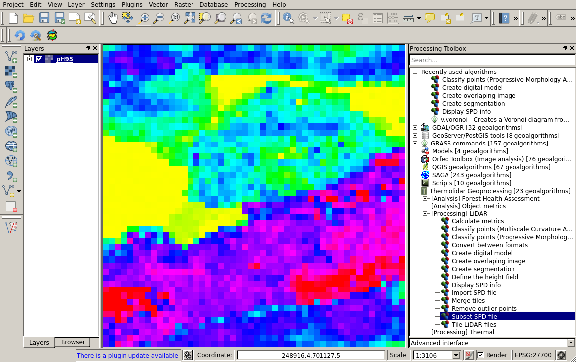
Height 95th percentile computed into a raster image (10m resolution)

4.3. Statistics¶

To measure tree biological and physical properties (e.g. dominant height, mean diameter, stem number, basal area, timber volume, etc...) throughout an entire woodlands is impossible. For this reason, only a few sample plots are usually measured in field in order to related them to canopy height metrics derived from LiDAR data. These relationships are then used to estimate and extend those characteristics to the area covered by LiDAR data and create forest inventory cartography. Two different models have been implemented in the ThermoLiDAR plug-in.

4.3.1. Stepwise Multivariate Regression Model¶

The Stepwise Multivariate Regression model was firstly introduce by Naesset (1997a, 1997b) to estimates tree heights ([Naesset1997a]) and volumes ([Naesset1997b]). The methodology assumes that stands have been previously classified before sample plots are measured. Plots must have the same size and have to be regularly distributed throughout the study area. Height metrics derived from LiDAR have to be calculated within each single sample plot (see Generate metrics) excluding points lower than 2 meters, so that stones and shrubs are avoided. Metrics have to include (Naesset 2002; [Naesset2002]):

Quantiles corresponding to the 0th, 5th, 10th, 15th, ..., 90th, 95th, 98th percentiles of the distribution.
The maximum values
The mean values
The coefficients of variation
Measures of canopy density

Naesset definition of canopy density is considered as the proportions of the first echo laser hits above 0th, 10th, ..., 90th percentiles of the first echo height distribution to total number of first echos.

For each sample plot a logarithmic regression equation is formulated:

\[Y = \beta_0 h_0^{\beta_1} h_{10}^{\beta_2} \ldots h_{90}^{\beta_{11}} h_{max}^{\beta_{12}} h_{mean}^{\beta_{13}} d_{10}^{\beta_{14}} \ldots d_{90}^{\beta_{23}} \ldots\]

which, in linear form is expressed as:

\[\begin{split}\ln Y &= \ln\beta_0 + \beta_1 \ln h_0 + \beta_2 \ln h_{10} \ldots + \beta_{11} \ln h_{90} + \beta_{12} + \\ &+ \ln h_{max} + \beta_{13} \ln h_{mean} + \beta_{14} \ln d_{10} + \ldots + \beta_{23} \ln d_{90}^{\beta_23} + \ldots\end{split}\]

Where \(Y\) are the field values (dependent variable); \(h_{i}\) are height percentiles; \(h_{max}\) and \(h_{mean}\) are maximum and mean height, respectively; and \(d_{j}\) are Naesset canopy densities.

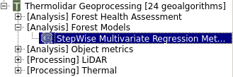
../_images/Toolbox_multivariate_regression.png

The module to calibrate the the forest model is located in [Analisis] Forest Model submenu of the ThermoLiDAR toolbox

4.3.1.1. Parameters¶

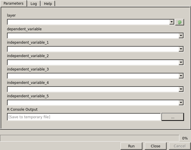
../_images/Module_multivariate_regression.png

Interface to calculate calibrate the forest model

4.3.1.1.1. Required Input Parameters¶

Layer: Shapefile layer that contains the LiDAR metrics.
Dependent Variable: Vector field containing the observations of the predictable variable
Independent Variable i: Vector field containing the LiDAR metrics that will be use to characterized the model

4.3.1.1.2. Output Parameters¶

Output: (html) File containing the final report of the multivariate regression

4.4. Forest Health Assessment¶

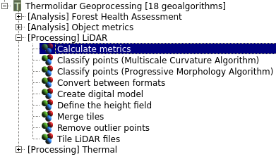
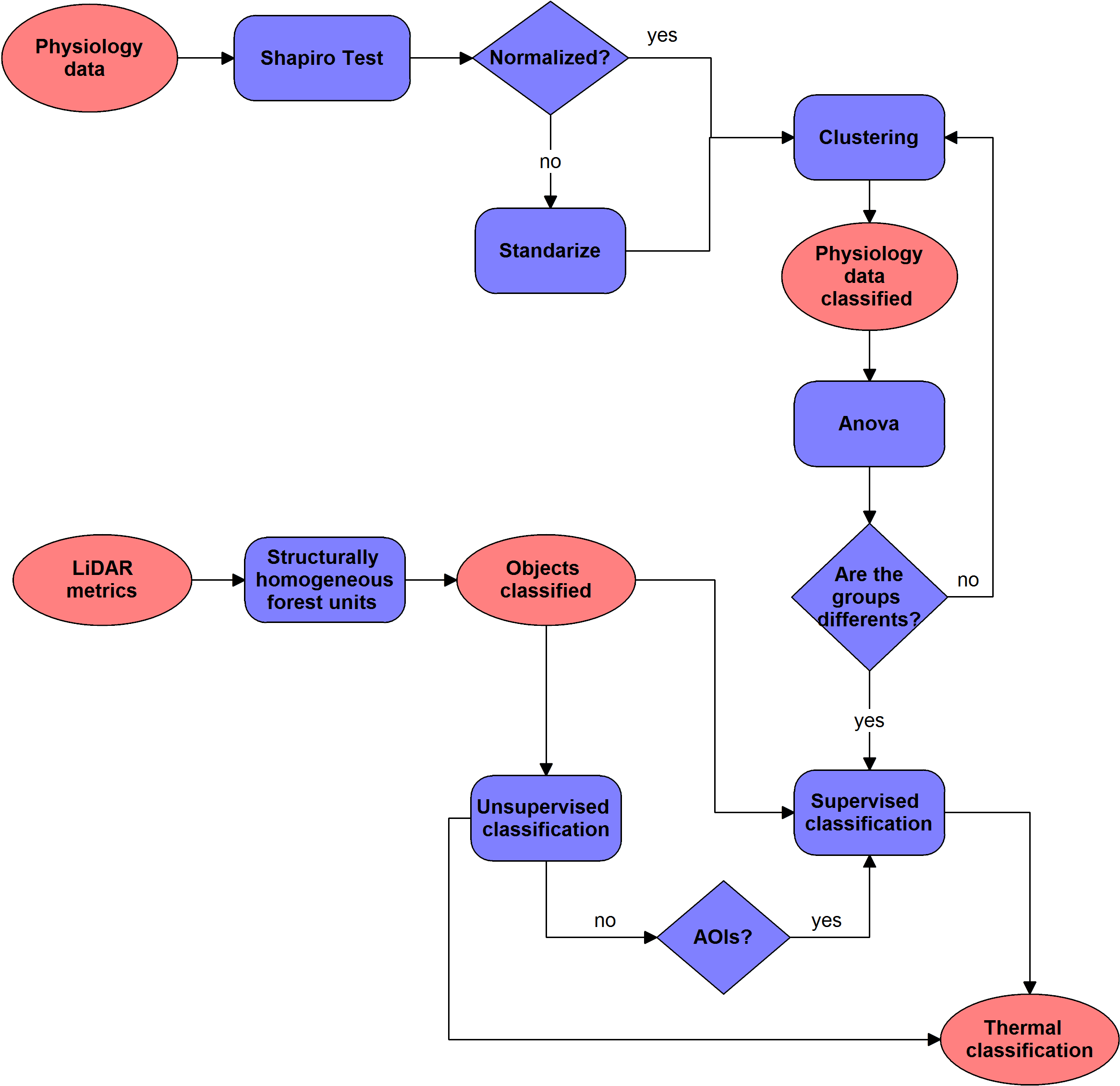
Forest Health assessment module consists of four different tools: Forest Stand Segmentation (FSS), Health Condition Level (HCL), Structurally Homogeneous Forest Units (SHFU) and Forest Health Monitoring (FHM). The following figure summarizes the main structure of this module and the input required throughout the process.

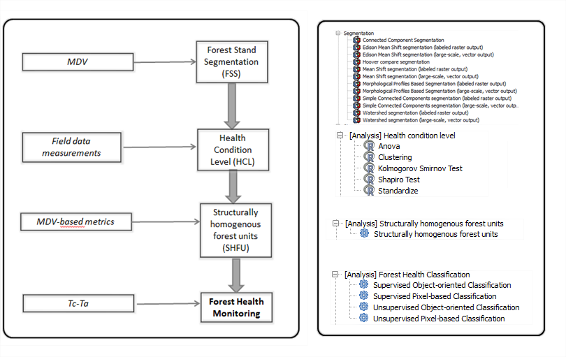
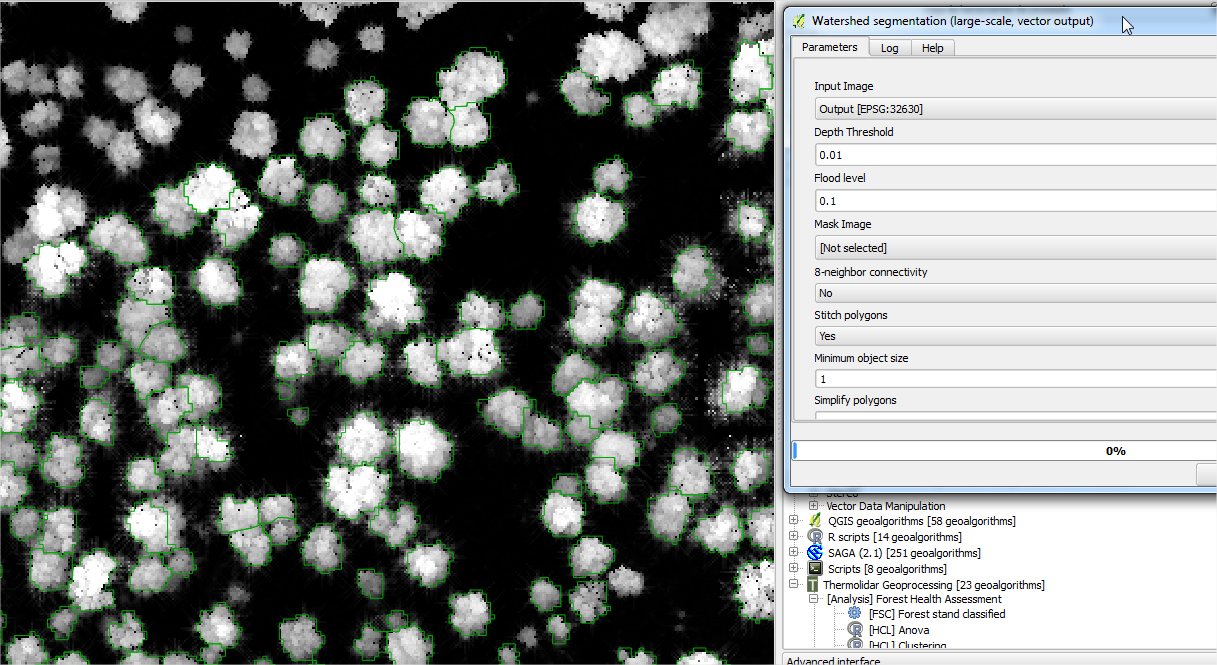
4.4.1. Forest stands segmentation¶

Within OD tools, users are willing to choose between developing a semi-automatic segmentation and using a pre-defined object feature. Segmentation tools are based on algorithms that segment an image into areas of connected pixels based on the pixel DN value. ThermoLiDAR image segmentation tools will be based on region growing algorithms. The basic approach of a region growing algorithm is to start from a seed region (typically one or more pixels) that are considered to be inside the object to be segmented. The pixels neighbouring this region are evaluated to determine if they should also be considered part of the object. If so, they are added to the region and the process continues as long as new pixels are added to the region. Region growing algorithms vary depending on the criteria used to decide whether a pixel should be included in the region or not, the type connectivity used to determine neighbours, and the strategy used to visit neighbouring pixels. Image segmentation is a crucial step within the object-based remote sensing information retrieval process. As a step prior to classification the quality assessment of the segmentation result is of fundamental significance for the recognition process as well as for choosing the appropriate approach and parameters for a given segmentation task. Alternatively, user could be interested on using a pre-defined object feature. This object feature could be a segmentation shape file provided from other source or any other land cover mapping. Also, the user can use a pre-defined regular object, defining the size of the square to be used previously.

4.4.2. Forest Condition Levels¶

The most critical part in applying forest health condition indicators is the user’s accuracy defining forest degradation levels. Besides user’s training another critical factor is to select under analysis a robust physiological indicator and to carry out an accurate field measurements campaign.

Potential physiological indicators of forest decline such us pigment concentration, photosynthesis, respiration and transpiration rate holds great potential to shed light on the mechanisms and processes that occur as a result of drought stress. In the short-term, climate can change the physiological conditions of the forest resulting in acute damage, but chronic exposure usually results in cumulative effects on physiological process. These factors effects on the plants light reactions or enzymatic functions and increased respiration from reparative activities. Gradual decreases in photosynthesis, stomatal conductance, carbon fixation, water use efficiency, resistance to insect and cold resistance were found in most of trees which are very typical symptom of stress conditions

Long-term exposure of water stress to a combination of high light levels and high temperatures causes a depression of photosynthesis and photosystem II efficiency that is not easily reversed, even for water-stress-resistant forest species. The decrease in the photochemical efficiency of photosystem II (ΦPSII) is related to the conversion of violaxanthin to antheraxanthin and zeaxanthin produced by an increase in harmless non-radiative energy dissipation (qN) and providing photo-protection from oxidative damage. One of the most widely physiological indicator applied in the analysis of long-term effect on forest health condition is de Leaf Area Index (LAI). The following is an example of the statistical analysis performs on LAI values measured from an Oak forest inventoried in the framework of THERMOLIDAR project.

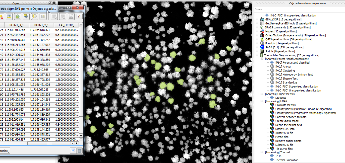
4.4.3. Structurally Homogeneous Forest Units¶

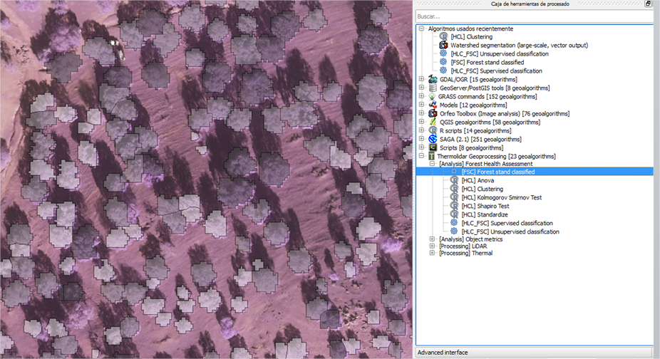
This tool provides the tools required for the classification of forest stands structurally different. The classification is based on two main structural parameters, average height of the trees and density. Input data needed to run this process is obtained from Lidar data. Alternatively, user can provide external forest maps in a .shp format type with an attribute of the number of class. The following figure shows an example of the units defined for the oak forest under analysis. Using a grey scale, trees were grouped in 3 classes with significant differences in terms of structural composition.

4.4.4. Forest Health Monitoring¶

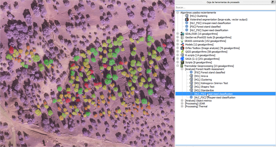
The main function of this tool is defining health condition differences in the vegetation at the stand level. Input parameters defined by users should mainly contain: thermal imaging data and the FSC Polygons (vector file with structurally homogeneous stands. Forest stands included in this analysis should be carried specifically based on one species. The user can perform a supervised or an unsupervised classification depending of the availability of field data measurements to define training areas. It should be highlight, that at this point of the analysis, users are willing to obtain an integrated mapping of forest health distribution levels based on thermal data but also standardized by forest stands units defined from lidar-based metrics. The following figure, shows an example of the units defined for assessment of the status of forest condition. Using a colour palette, trees were grouped in different classes with significant differences in terms of structural composition and physiological status. The colour palette ranges from red to green, where red colour is relate with trees with high level of damage and green colour represents trees with optimum health condition.

4.5. Data Analysis¶

This section provides the tools for analysis and interpretation of results. Once thermal and LiDAR data have been processed in the previous sections, the user can generate the mapping needed to interpret the physiological state of the forest mass analysed. First, the user has a set of data obtained in the field of physiology which are analysed and grouped, using the tools available at the module Health Condition Level. From the tools available in the structurally homogeneous forest units module, the user can perform a preliminary classification of the stands, based on structural homogeneity. This factor is important because thermal values behave differently according to the structure of objects. Finally, from the Forest Heath classification tools the user has the necessary tools to perform a classification based on the thermal values for the various homogeneous units. To improve the classification, the user can define training plots according to data collected in the field of physiology, visually are established different levels of affection.

4.5.1. Health Condition Levels¶

4.5.1.1. Shapiro Test¶

Before proceeding with the classification of items by level of damage according to several variables taken in the field, we verify that the set of physiological variables follow a normal distribution. For this we use the Shapiro test, located in the toolbox [Analysis] Health Condition Level > Shapiro Test.

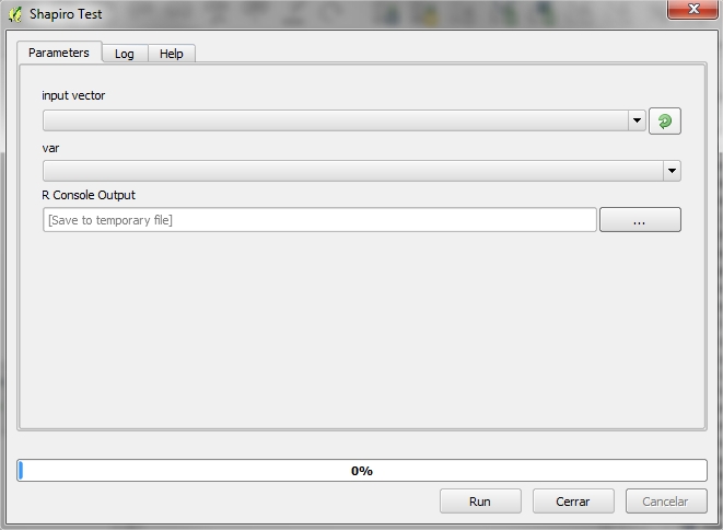
4.5.1.1.1. Required Input Parameters¶

Input vector: Vector file that contains information on physiological data.
Parameter: Vector’s field to analyze if it follows the normal distribution

4.5.1.1.2. Ouput Parameters¶

R Console Output: File with the output result. The output is composed of the following values
- Statistic - The value of the Shapiro-Wilk statistic.
- p.value - An approximate p-value for the test. This is said in Royston (1995) to be adequate for p.value < 0.1.
- Method - The character string “Shapiro-Wilk normality test”.
- data.name - A character string giving the name(s) of the data.

4.5.1.2. Interpretation¶

The null-hypothesis of this test is that the population is normally distributed. Thus if the p-value is less than the chosen alpha level, then the null hypothesis is rejected and there is evidence that the data tested are not from a normally distributed population. In other words, the data is not normal. On the contrary, if the p-value is greater than the chosen alpha level, then the null hypothesis that the data came from a normally distributed population cannot be rejected. E.g. for an alpha level of 0.05, a data set with a p-value of 0.02 rejects the null hypothesis that the data are from a normally distributed population. However, since the test is biased by sample size, the test may be statistically significant from a normal distribution in any large samples.

4.5.1.3. Standardize¶

To be able to use the variables in our analysis, they should follow a normal distribution. One way to force these follow a normal distribution is by definition. This characterization involves the conversion of the variable that follows a distribution N (μ, σ), a new variable with distribution N (1,0). This tool is situated in [Analysis] Heath condition level > Standardize.

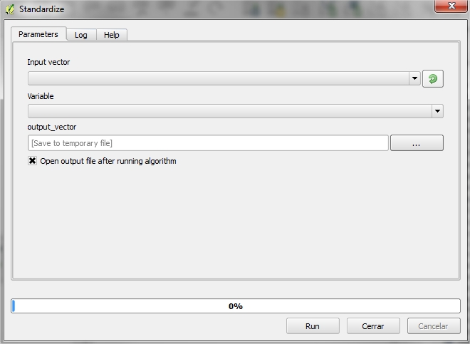
4.5.1.3.1. Required Input Parameters¶

Input vector: Shape that contains information on physiological data.
Variable: Shapefile’s field to standardize

4.5.1.3.2. Ouput Parameters¶

Output vector: The user will output a new shapefile with the standardized variable.

4.5.1.4. Clustering¶

This tool allows us to group one or more physiological variables according to their degree of similarity between individuals in the sample. So, the goal of clustering is to determine the intrinsic grouping in a set of unlabelled data. But how to decide what constitutes a good clustering? It can be shown that there is no absolute best criterion which would be independent of the final aim of the clustering. Consequently, it is the user which must supply this criterion, in such a way that the result of the clustering will suit their needs. To make this tool has been chosen by a hierarchical approach. The user-supplied items are categorized into levels and sublevels within a class hierarchy, forming a hierarchical tree structure.

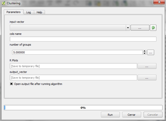
4.5.1.4.1. Required Input Parameters¶

Input vector: Shape containing information on physiological data.
Cols names: Name the columns containing details physiology (separated by semicolons ‘;’)
Number of groups: Number of groups

4.5.1.4.2. Ouput Parameters¶

R plots: File with the R output result.

Output vector: Output shapefile with a new variable (group) indicating that each group is member.

4.5.1.5. ANOVA¶

ANOVA test are conducted for each variable to indicate how well the variable discriminates between clusters. The hypothesis is tested in the ANOVA is that the population means (the average of the dependent variable at each level of the independent variable) are equal. If the population means are equal, it means that the groups did not differ in the dependent variable, and consequently, the independent variable is independent of the dependent variable.

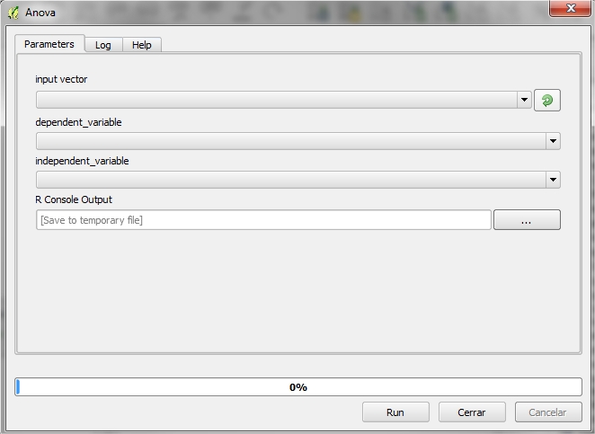
4.5.1.5.1. Required Input Parameters¶

Input vector: Shapefile that contains information about the cluster
Dependent variable: Field shape that acts as a dependent variable
Independent variable: Field shape that acts as an independent variable

4.5.1.5.2. Ouput Parameters¶

R Console Output: File with the R output result. The result will be a list of ANOVA tables, one for each response (even if there is only one response”. They have columns “Df”, “Sum Sq”, “Mean Sq”, as well as “F value” and “Pr(>F)” if there are non-zero residual degrees of freedom. There is a row for each term in the model, plus one for “Residuals” if there are any.

4.5.1.6. Interpretation¶

If the critical level associated with the F statistics (ie, the probability of obtaining values as obtained or older), is less than 0.05, we reject the hypothesis of equal means and conclude that not all the population means being compared are equal. Otherwise, we cannot reject the hypothesis of equality and we cannot claim that the groups being compared differ in their population averages.

4.5.2. Structurally Homogeneous Forest Units¶

4.5.2.1. Structurally Homogeneous forest units¶

The analytical purpose of this tool is the definition of structurally homogeneous stands that allow us to minimize the effects of structure on the thermal information, and therefore allow us to obtain related health outcomes woodland. To do this, the software allows the user to define the structure of the stand from the height data. The calculation of uniformity is therefore a function of two variables directly derived from LiDAR data the 95th percentile obtained from MDV and the penetration rate, obtained from density points that penetrate the forest canopy.

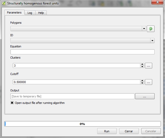
4.5.2.1.1. Required Input Parameters¶

Polygons: Vector file that contains polygons to classify.
ID: Vector’s field that that indicates the id of each item
Equation: Operator used to classify the feats.
Clusters: Number of output groups. The value is 3 by default.
Cutoff: Stop threshold algorithm. The value is 0.5 by default.

4.5.2.1.2. Ouput Parameters¶

Output: Vector file name containing the classification.

4.5.3. Forest Health Classification¶

4.5.3.1. Unsupervised Pixel-based Classification¶

The user has a stratification of the study area, and classified based on the structure. Through this tool, a classification of the pixels of temperatures will be performed, based on the classification of defined structure. Thus, the output will be a raster temperature for each of the groups of homogeneity.

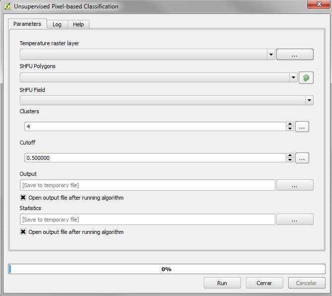
4.5.3.1.1. Required Input Parameters¶

Temperature raster layer: Input temperature raster
SHFU Polygons: Vector layer that contains structurally homogenous stands.
SHFU Field: SHFU layer field containing the group that belong each item.
Clusters: Number of output classes.
Cutoff: Stop threshold. The value is 0.5 by default.

4.5.3.1.2. Ouput Parameters¶

Output: Raster file name containing the classification of temperatures based on homogenous stand units.
Statistics: CSV File containing statistics for groups.

4.5.3.2. Unsupervised Object-oriented Classification¶

The user has a stratification of the study area, and classified based on the structure. Through this tool, a classification of the objects of temperatures mean will be performed, based on the classification of defined structure. Thus, the output will be a raster temperature for each of the groups of homogeneity.

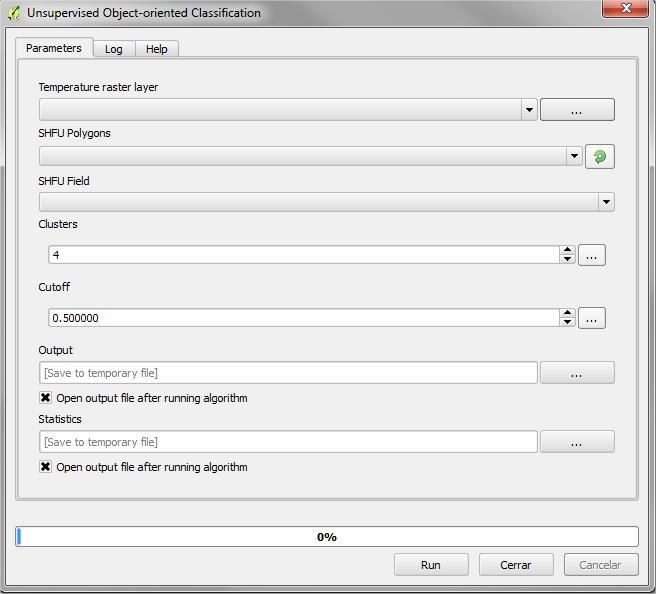
4.5.3.2.1. Required Input Parameters¶

Temperature raster layer: Input temperature raster
SHFU Polygons: Vector layer that contains structurally homogenous forest units.
SHFU Field: SHFU layer field containing the group that belongs each item.
Clusters: Number of output classes.
Cutoff: Stop threshold. The value is 0.5 by default.

4.5.3.2.2. Ouput Parameters¶

Output: Raster file name containing the classification of temperatures based on homogenous stand units.
Statistics: CSV File containing statistics for groups.

4.5.3.3. Supervised Pixel-based Classification¶

Similarly as in the previous point, the user can perform a classification of the temperature response to the stand of homogeneity. Unlike supervised classification, the user has a number of AOIs that guide the classification process.

4.5.3.3.1. Required Input Parameters¶

Temperature raster layer: Input temperature raster
SHFU Polygons: Vector layer that contains structurally homogenous stands.
SHFU Field: SHFU layer field containing the group that belong each item.
ROIs vector: Vector file with training areas.
ROIs - SHFU Identifier: Vector’s field that contains the group’s homogeneity that belongs each item of training areas.
ROIs - FSC Identifier: Vector’s field that contains the group “Forest health level” that belongs within their group of homogeneity.
k: Number k nearest neighbors. The value is 3 by default.

4.5.3.3.2. Ouput Parameters¶

Output: Raster file name containing the classification of temperatures based on homogenous stand units.

Statistics: CSV File containing statistics for groups.

4.5.3.4. Supervised Object-oriented Classification¶

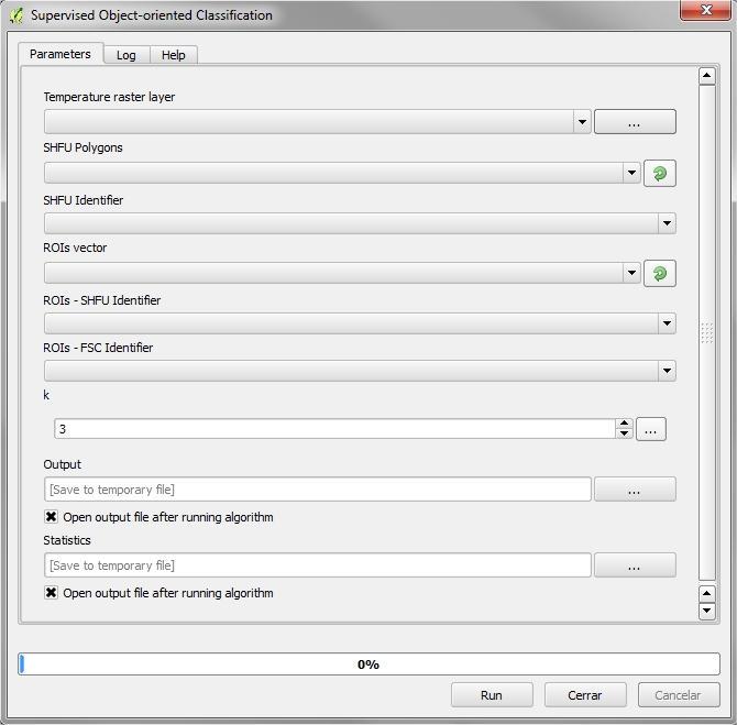
4.5.3.4.1. Required Input Parameters¶

Temperature raster layer: Input temperature raster
SHFU Polygons: Vector layer that contains structurally homogenous stands.
SHFU Field: SHFU layer field containing the group that belong each item.
ROIs vector: Vector file with training areas.
ROIs - SHFU Identifier: Vector’s field that contains the group’s homogeneity that belongs each item of training areas.
ROIs - FSC Identifier: Vector’s field that contains the group “Forest health level” that belongs within their group of homogeneity.
k: Number k nearest neighbors. The value is 3 by default.

4.5.3.4.2. Ouput Parameters¶

Output: Raster file name containing the classification of temperatures based on homogenous stand units.
Statistics: CSV File containing statistics for groups.

References

[Bunting2013]

Bunting, P., Armston, J., Clewley, D., Lucas, R. M., 2013. Sorted pulse data (SPD) library. Part II: A processing framework for LiDAR data from pulsed laser systems in terrestrial environments. Computers and Geosciences 56, 207 – 215.

[BaterCoops2009]

Bater, C. W., Coops, N. C., 2009. Evaluating error associated with lidar-derived DEM interpolation. Computers and Geosciences 35 (2), pp. 289–300.

[EvansHudak2007]

Evans, J. S., Hudak, A. T., 2007. A multiscale curvature algorithm for classifying discrete return lidar in forested environments. IEEE Transactions on Geoscience and Remote Sensing 45 (4), pp. 1029 – 1038.

[Naesset1997a]

Naesset, E., 1997. Determination of mean tree height of forest stands using airborne laser scanner data. ISPRS Journal of Photogrammetry and Remote Sensing, 52, pp. 49 – 56.

[Naesset1997b]

Naesset, E., 1997. Estimating timber volume of forest stands using airborne laser scanner data. Remote Sensing of Environment, 61, pp. 246 – 253.

[Naesset2002]

Naesset, E., 2002. Predicting forest stands characteristics with airborne scanning laser using a practical two-stage procedure and field data. Remote Sensing of Environment, 80, pp. 88 – 99.

[Zhang2003]

Zhang, K., Chen, S., Whitman, D., Shyu, M., Yan, J., Zhang, C., 2003. A progressive morphological filter for removing nonground measurements from airborne LIDAR data. IEEE Transactions on Geoscience and Remote Sensing 41 (4), pp. 872 – 882.