5. Examples
5.1. Case Study 1 - Huelva (Spain)
5.1.1. Thermal Processing
5.1.1.1. Thermal Calibration
For calibration of the thermal image we have the following data:
- Thermal image of the study area in Huelva, each pixel of the image represents the temperature value in degrees kelvin. thld_training\huelva\Z1_holmOak\Temperature\t_huelvaZ1.tif
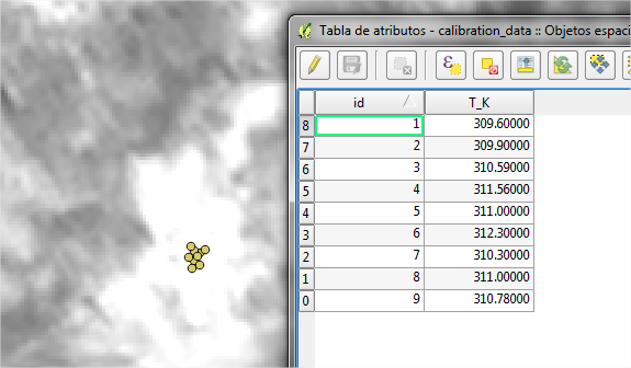
- Set of calibration values stored in a vector file. Each item has the id and the value of collected temperature (in degrees Kelvin). thld_training\huelva\Z1_holmOak\Temperature\t_aois\t_calibration.shp
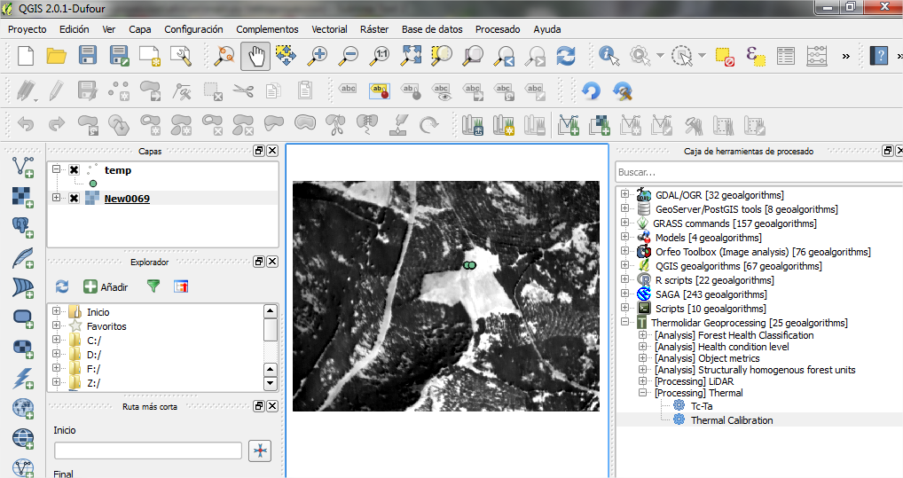
We proceed to load both the image and the shape to QGIS interface. To load the image in the main menu (Layer - Add Raster Layer ...) to load the shape of points (Layer - Add Vector Layer ...).
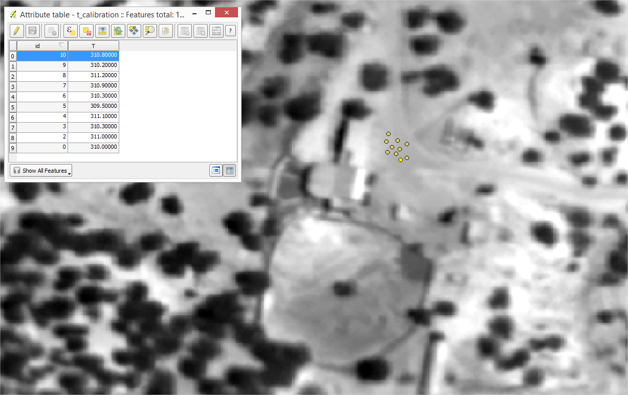
Thermal image of Huelva and attribute table containing the field thermal data
We proceed to perform the calibration of the thermal image through Thermolidar tool toolbox [Processing] Thermal - Thermal Calibration.
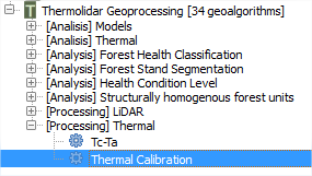
Thermal calibration tool
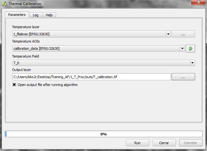
We introduce the values as shown in the interface:
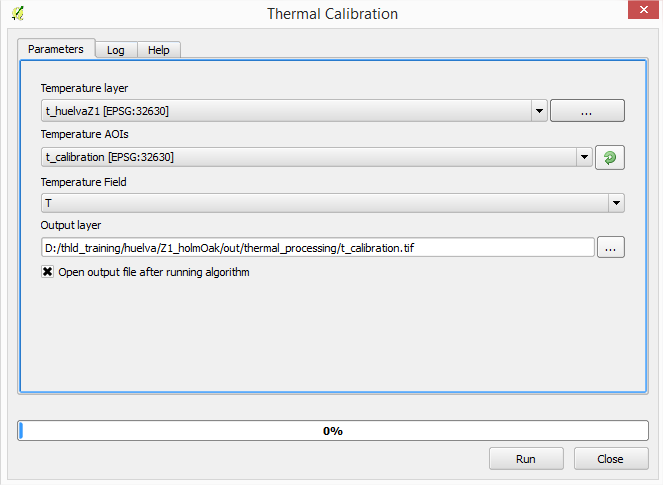
Interface of the Thermal Calibration module
We obtain as output calibration file of the thermal image, as shown in the following figure:
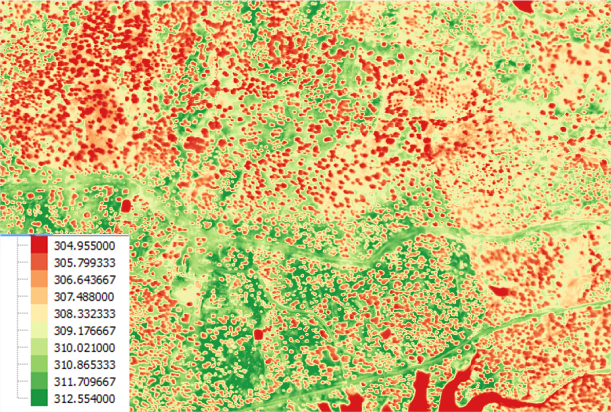
Thermal calibration output
5.1.1.2. Tc - Ta
We proceed to subtract the air temperature to the calibrated raster temperatures. We have available the following information.
- Raster temperature calibrated in the previous section. thld_training\huelva\Z1_holmOak\out\thermal_processing\t_calibration.tif
- Air temperature acquired in flight time. In our case we will use the value of temperature 298.15 ºK
We proceed to perform the calibration of the thermal image through Thermolidar tool toolbox [Processing] Thermal - Tc-Ta.
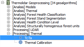
Tc Ta module is located in the “Thermal” submenu of the THERMOLIDAR plugin toolbox
We introduce the input parameters in the user interface:
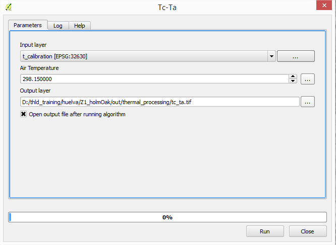
Interface of the Tc-Ta module
Obtaining as output file the following result:
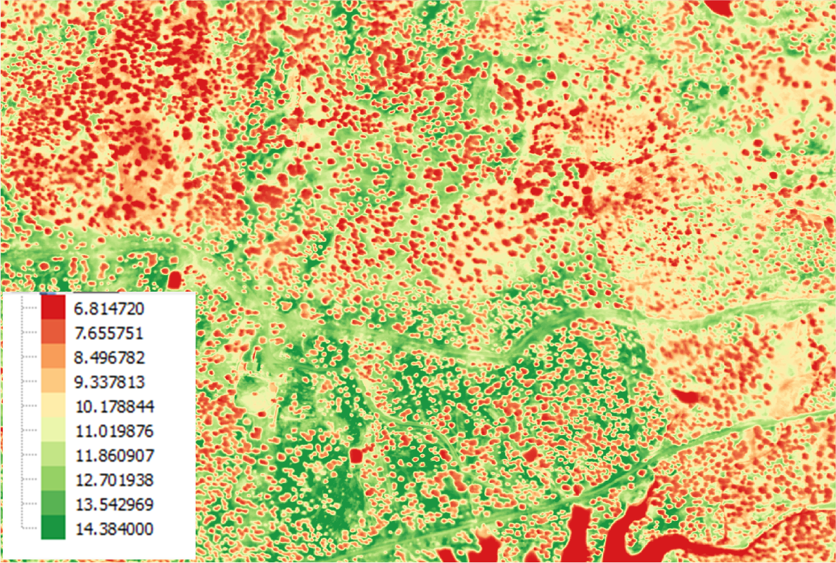
Output thermal image of Huelva
5.1.2. Data analysis
5.1.2.1. Health condition levels
We have the physiology data of Leaf Area Index (LAI) for 25 of the 216 trees inventoried in the area of Huelva, stored in the vector file: thld_training\huelva\Z1_holmOak\FieldData\LAI\lai_huelva.shp.
First, load the shape of polygons in QGIS (Layer - Add vector layer ...)
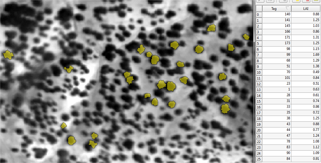
LAI measurements in Huelva
Before proceeding with the classification of items by level of damage according to several variables taken in the field, we verify that the set of physiological variables follow a normal distribution. For this we use the Shapiro test, located in the toolbox [Analysis] Health Condition Level > Shapiro Test.
Warning
The first time you use these tools, you will need to start QGIS in administrator mode (R install required dependencies)
5.1.2.2. Shapiro Test
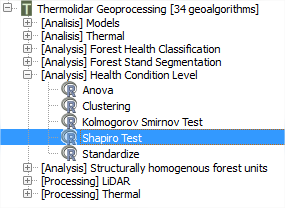
Shapire Test is located in the “Health Condition Level” submenu of the THERMOLIDAR plugin toolbox
- Input vector: Vector file that contains information on physiological data.
- Var: Vector’s field to analyze if it follows the normal distribution. In this case the parameter LAI
We introduce the parameters as shown in the following figure:
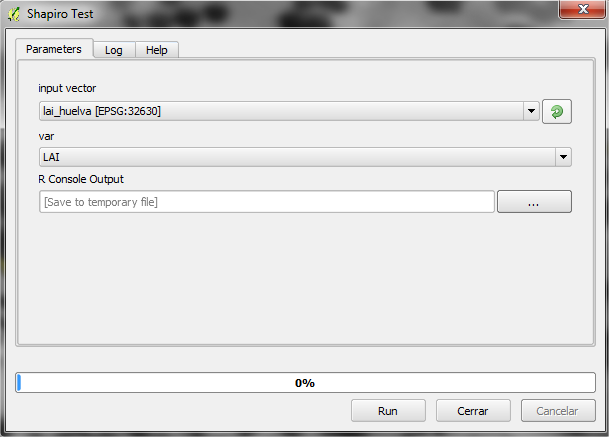
Interface of the “Shapiro Test” module
Obtaining the following output:
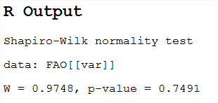
In the example, the p-value is much higher than 0.05, so we conclude that LAI data follow a normal distribution. In the case where p-value is less than 0.05 the data would be discarded, or these should be normalized.
In the case that the variable does not follow a normal distribution, it is necessary to standardize using the [Analysis] Health Condition Level> Standarize
5.1.2.3. Clustering
This tool allows us to group one or more physiological variables according to their degree of similarity between individuals in the sample. In this case we will group by the variable LAI, we have previously verified that follows a normal distribution. This tool creates many groups tool damage level depending on the specified physiological variable. In this case, we will select 3 levels as a function of LAI variable. We can find the tool in [Analysis] Health Condition Level > Clustering
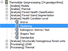
Clustering is located in the “Health Condition Level” submenu of the THERMOLIDAR plugin toolbox
We introduce the values as shown in the following figure:
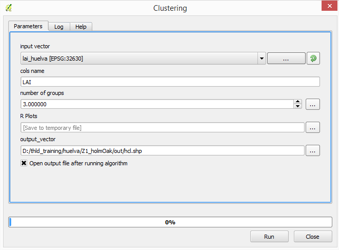
The vector output file will be stored in the folder thld_training\huelva\Z1_holmOak\out\hcl.shp that will be used subsequently. Each of the trees will be classified as regions of interest to guide the supervised classification of the thermal image.
We obtain results in the dendrogram with the cluster of data:
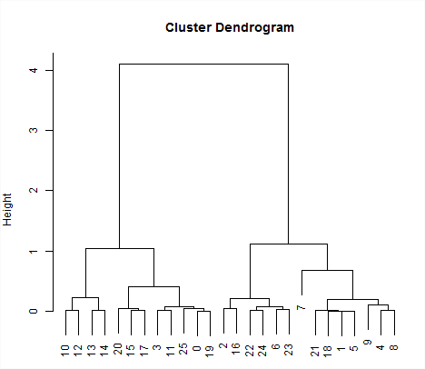
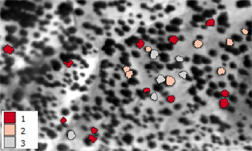
LAI data grouped into 3 categories health condition, with the following results:
Finally, we must ensure that the groups are significantly different, according to the variables used. This is done through the tool [Analysis] Heath condition level> ANOVA.
5.1.2.4. ANOVA
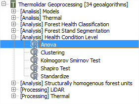
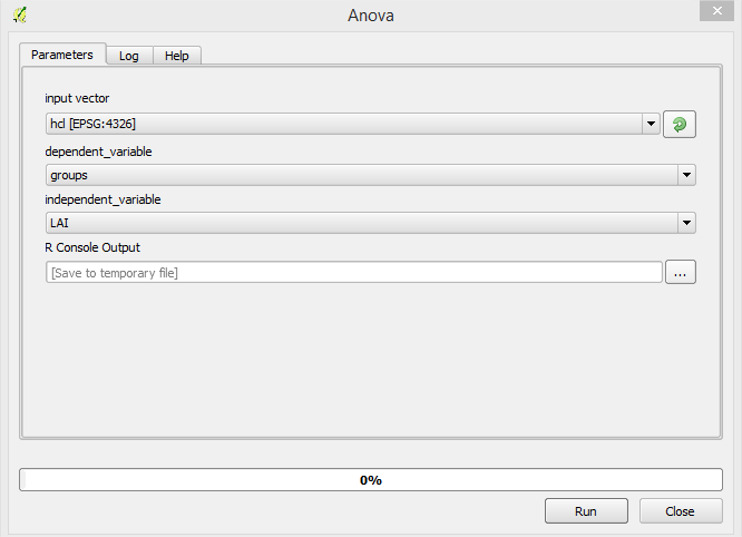
ANOVA is located in the “Health Condition Level” submenu of the THERMOLIDAR plugin toolbox
Selected as the dependent variable the group that owns each parcel; and as the dependent variable that we want to check if it is significant in the group.
We get the following output:
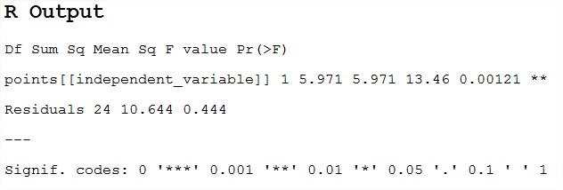
If the critical level associated with the F statistics (ie, the probability of obtaining values as obtained or older), is less than 0.05, we reject the hypothesis of equal means and conclude that not all the population means being compared are equal. Otherwise, we cannot reject the hypothesis of equality and we cannot claim that the groups being compared differ in their population averages.
5.1.2.5. Structurally homogenous forest units
The analytical purpose of this tool is the definition of structurally homogeneous stands that allow us to minimize the effects of structure on the thermal information, and therefore allow us to obtain related health outcomes woodland.
We start from the metric of the objects to be classified. This vector file was generated at the point of obtaining metric lidar [Processing] LiDAR > Calculate metrics.
- thld_training\huelva\Z1_holmOak\out\metrics.shp
The user must enter the equation by which you want to group the stands, for example according to the equation of the dominant height. In our case, we use the equation obtained from the 95th percentile.
The tool used in this section is located in [Analysis] Structurally homogeneus forest units
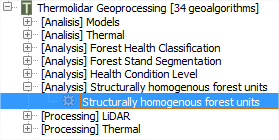
SHFU is located in the “Structuraly Homogeneous Forest Units” submenu of the THERMOLIDAR plugin toolbox
In this example, the polygons will be classified into 3 different groups of homogeneity (Cluster parameter).
The Cutoff parameter determines the accuracy of the fit. A value of 0 is of higher precision and larger number of iterations will be needed to reach the final solution.
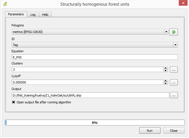
Interface of the “SHFU” module
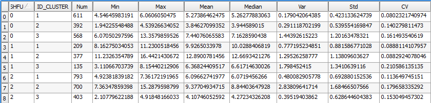
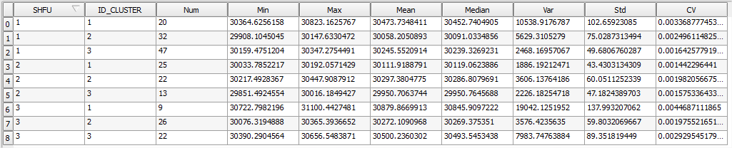
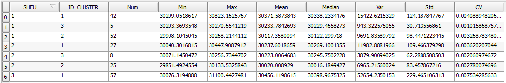
We get as output:
Now, we must assign the SHFU group to the objects (regions of interest) described on the Forest Health Level section.
Thus we will use vector files: * thld_training\huelva\Z1_holmOak\out\hcl.shp * thld_training\huelva\Z1_holmOak\out\shfu.shp
We will use the tool Vector > Data Management Tools > Join attributes by location
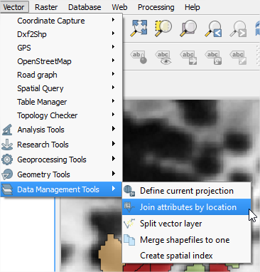
We insert the parameters as shown in the following figure:
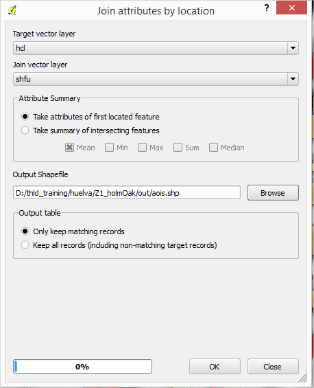
We will obtain a new output file (thld_training\huelva\Z1_holmOak\out\aois.shp) will use to guide the classification of the thermal image, are of interest to the following fields: • SHFU. Homogeneous group that the object owns. • Groups. Health condition level
5.1.2.6. Forest Health Classification
We proceed to perform the classification of the thermal image, based on the following information available:
- **thld_training\huelva\Z1_holmOak\Temperature\t_huelvaZ1.tif
- thld_training\huelva\Z1_holmOak\out\shfu.shp
For supervised classification we will use health condition levels obtained in previous sections.
- **thld_training\huelva\Z1_holmOak\out\aois.shp
5.1.2.7. Unsupervised pixel-based classification
Through this tool raster classify the temperature as many classes as you specify. Temperature classification is performed based on homogeneous units, so many output raster have been defined as SHFU be obtained.
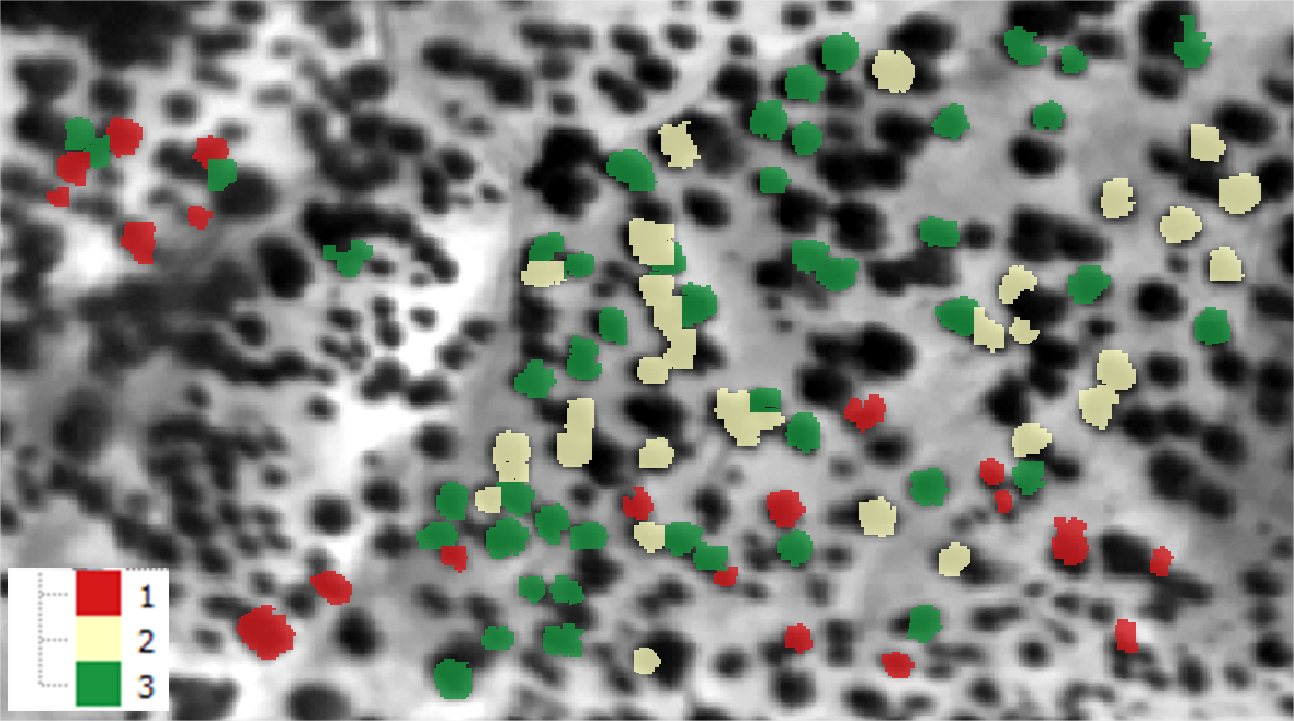
In our case, we obtain three raster classified. Each raster has associated many categories defined temperature.
Interface of the “Unsupervised pixel-based classification” module
We get as output:
5.1.2.8. Unsupervised object-based classification
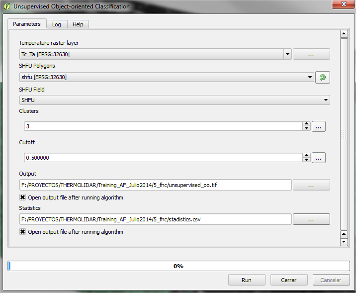
In the same way that the pixel-oriented, this tool classification raster classify the temperature as many classes as you specify. Temperature classification is performed based on homogeneous units, so many output raster have been defined as SHFU be obtained.
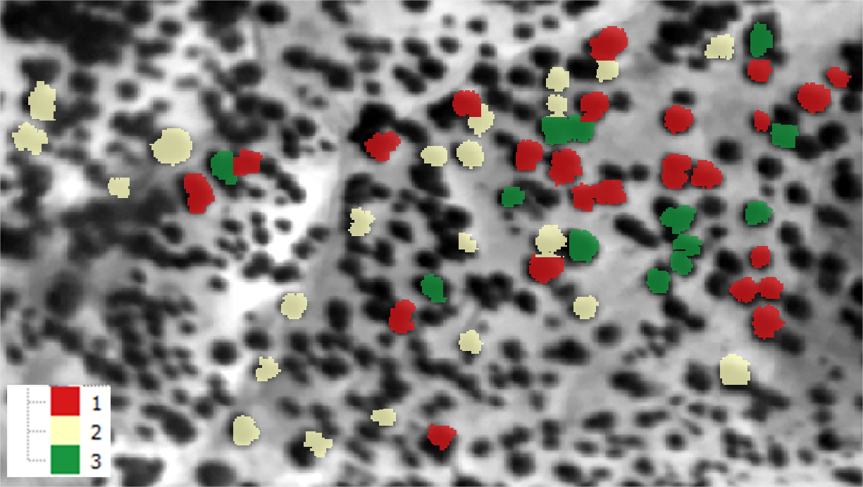
In our case, we obtain three raster classified. Each raster has associated many categories defined temperature.
The difference from the previous tool, is that instead of being classified pixels are classified objects. The classification is made based on the mean value of each of the objects.
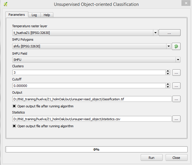
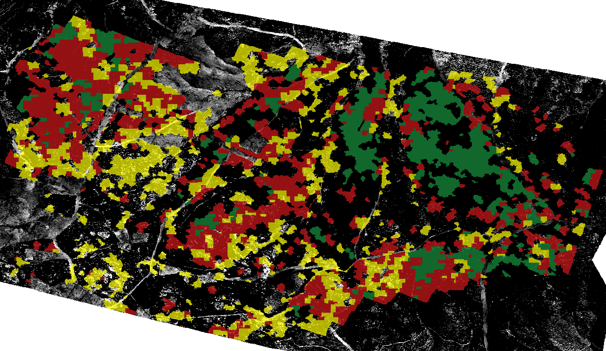
Interface of the “Unsupervised object-based classification” module
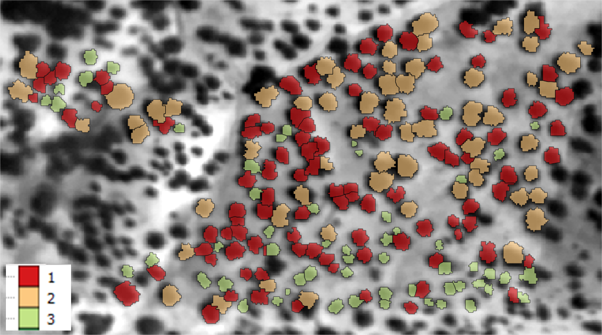
We get as output:
5.1.2.9. Supervised pixel-based classification
Through this tool the temperature raster will be classified, based on the condition levels defined in the regions of interest (AOIs). * **thld_training\huelva\Z1_holmOak\out\aois.shp
Temperature classification is performed based on homogeneous units, so many output raster have been defined as SHFU be obtained.
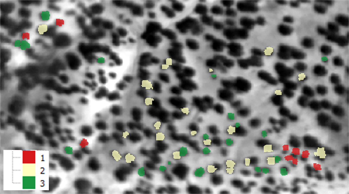
In our case, we obtain three raster classified. Each raster has associated many categories defined temperature.
Interface of the “Supervised pixel-based classification” module
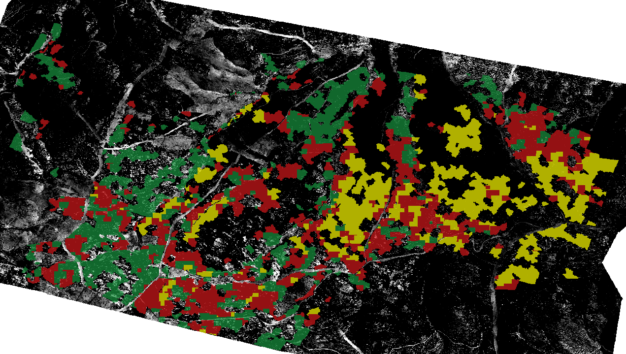
We get as output:
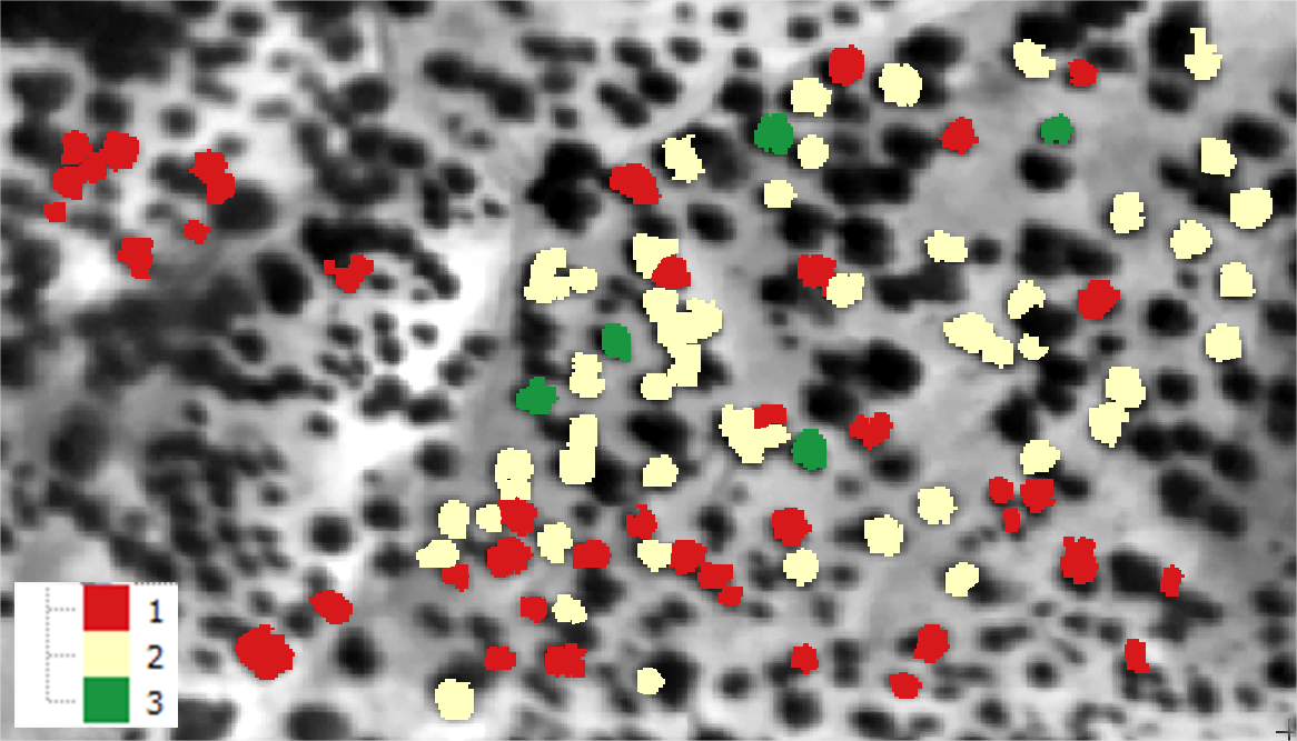
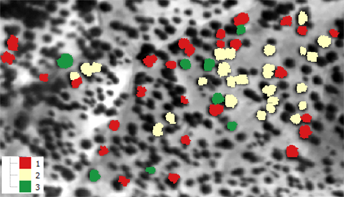
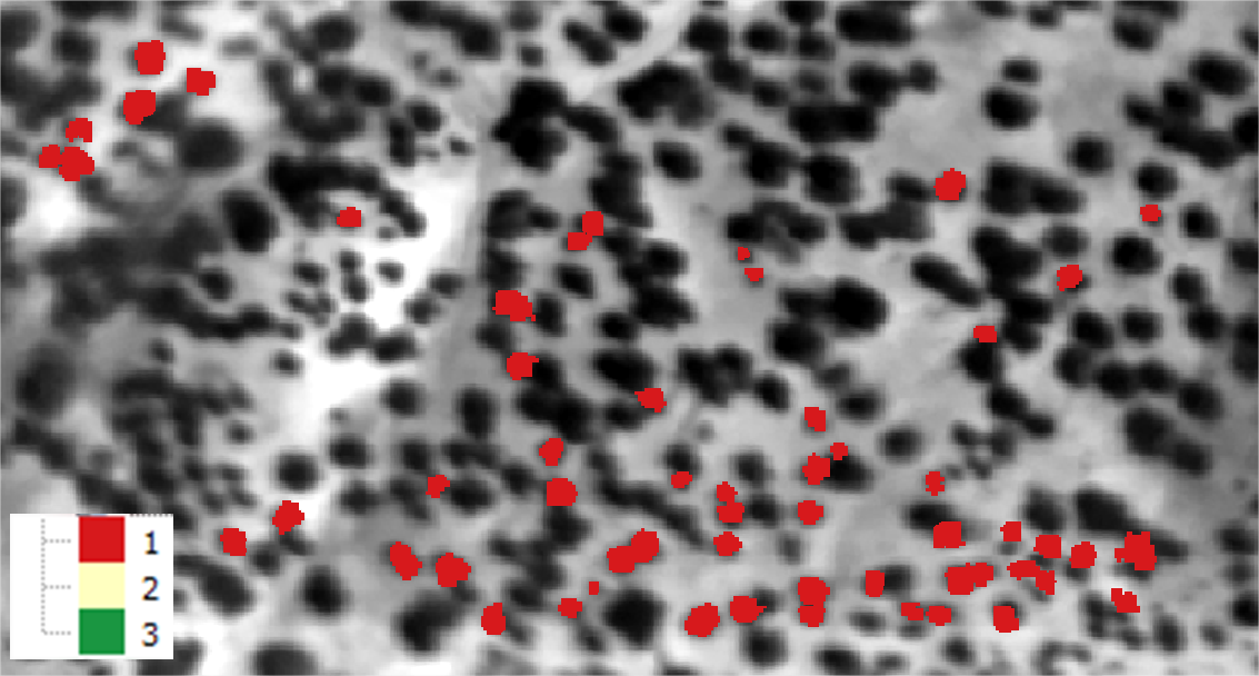
5.1.2.10. Supervised object-based classification
Through this tool the temperature raster will be classified, based on the condition levels defined in the regions of interest (AOIs). * **thld_training\huelva\Z1_holmOak\out\aois.shp
Temperature classification is performed based on homogeneous units, so many output raster have been defined as SHFU be obtained.
In our case, we obtain three raster classified. Each raster has associated many categories defined temperature.
The difference from the previous tool, is that instead of being classified pixels are classified objects. The classification is made based on the mean value of each of the objects.
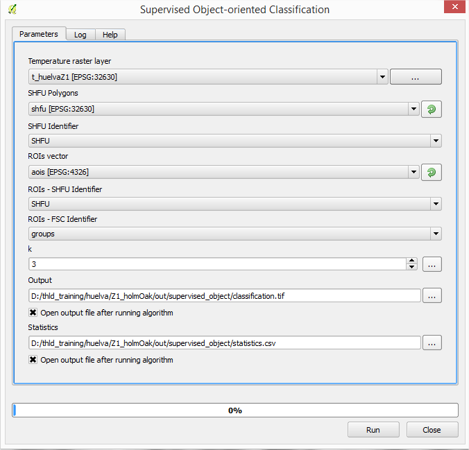
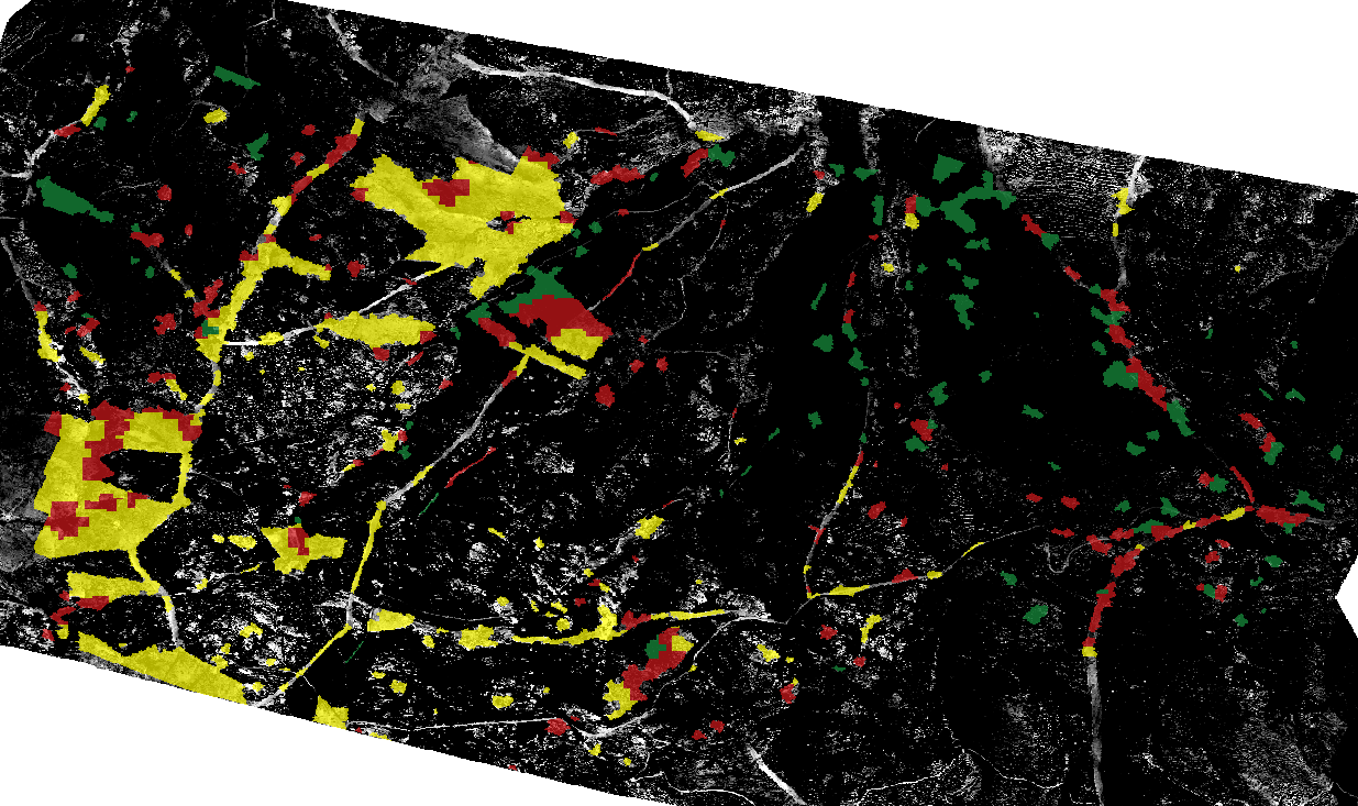
Interface of the “Supervised object-based classification” module
We get as output:
5.2. Case Study 2 - Almería (Spain)
5.2.1. Thermal Processing
5.2.1.1. Thermal Calibration
First, we have a thermal image of the study area. Each digital image value represents the temperature in degrees kelvin.
Thermal image of Sierra de los Filabres
Several values of temperature field of invariant surfaces (black and white cloth) have been collected, and GPS position of each sample.
Attribute table of shapefile containing the field thermal data.
We introduce the input parameters in the user interface:
Interface of the Thermal Calibration module
As a result the software generates a calibrated image of the study area.
5.2.1.2. Tc - Ta
We introduce the input parameters in the user interface:
- Input layer: Calibrated thermal raster (generated in the previous section)
- Air temperature: Constant air temperature measure at flight time. In this case, the air temperature is considered to 293.15 degrees kelvin
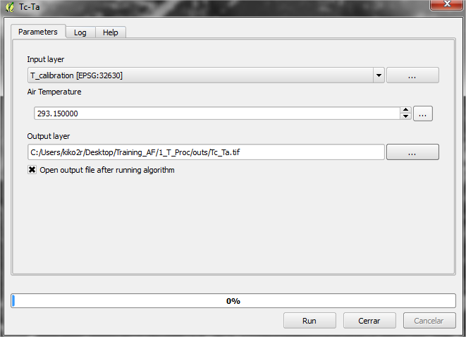
Interface of the Tc-Ta module
Output thermal image of Sierra de los Filabres
5.2.2. Data analysis
5.2.2.1. Health condition levels
In the following example we have acquired several variables physiology field (LAI), for a number of control plots in Filabres.
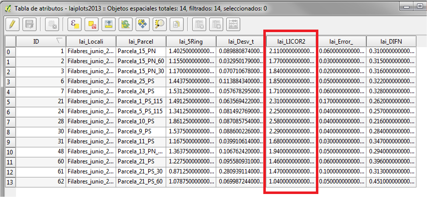
LAI measurements in Filabres
Before proceeding with the classification of items by level of damage according to several variables taken in the field, we verify that the set of physiological variables follow a normal distribution. For this we use the Shapiro test, located in the toolbox [Analysis] Health Condition Level > Shapiro Test.
Warning
The first time you use these tools, you will need to start QGIS in administrator mode (R install required dependencies)
5.2.2.2. Shapiro Test
- Input vector: Vector file that contains information on physiological data.
- Var: Vector’s field to analyze if it follows the normal distribution. In this case the parameter lai_LICOR2
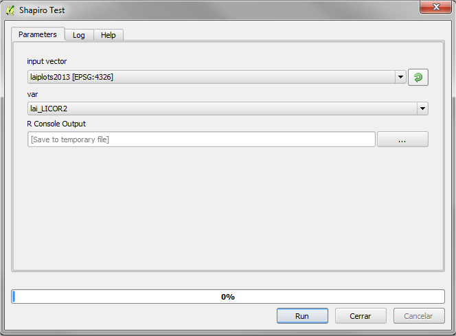
Interface of the “Shapiro Test” module
Obtaining the following output:
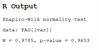
In the example, the p-value is much higher than 0.05, so we conclude that LAI data follow a normal distribution. In the case where p-value is less than 0.05 the data would be discarded, or these should be normalized.
In the case that the variable does not follow a normal distribution, it is necessary to standardize using the [Analysis] Health Condition Level> Standarize
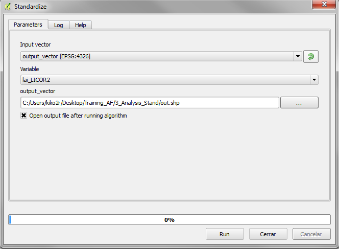
5.2.2.3. Standarize
We verified that the lai_LICOR2 variable follows a normal distribution.
- Input vector: Vector file that contains information on physiological data.
- Var: Shapefile’s field to standardize. In this case the parameter lai_LICOR2
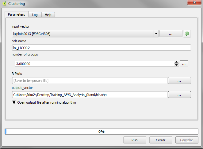
5.2.2.4. Clustering
This tool allows us to group one or more physiological variables according to their degree of similarity between individuals in the sample. In this case we will group by the variable lai_LICOR2, we have previously verified that follows a normal distribution. This tool creates many groups tool damage level depending on the specified physiological variable. In this case, we will select 3 levels as a function of LAI variable.
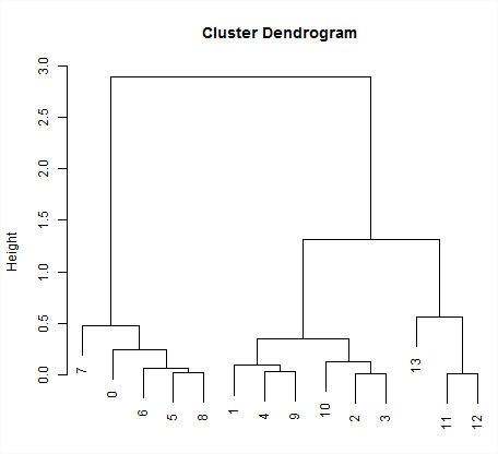
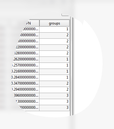
LAI data grouped into 3 categories health condition, with the following results:
Finally, we must ensure that the groups are significantly different, according to the variables used. This is done through the tool [Analysis] Heath condition level> ANOVA.
5.2.2.5. ANOVA
Selected as the dependent variable the group that owns each parcel; and as the dependent variable that we want to check if it is significant in the group.
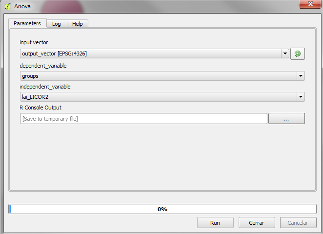
We get the following output:
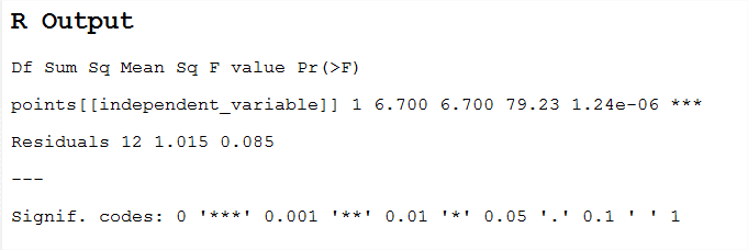
If the critical level associated with the F statistics (ie, the probability of obtaining values as obtained or older), is less than 0.05, we reject the hypothesis of equal means and conclude that not all the population means being compared are equal. Otherwise, we cannot reject the hypothesis of equality and we cannot claim that the groups being compared differ in their population averages.
5.2.2.6. Structurally homogenous forest units
The analytical purpose of this tool is the definition of structurally homogeneous stands that allow us to minimize the effects of structure on the thermal information, and therefore allow us to obtain related health outcomes woodland.
The user must enter the equation by which you want to group the stands, for example according to the equation of the dominant height. In our case, we use the equation obtained from the 95th percentile. In this example, the polygons will be classified into 3 different groups of homogeneity.
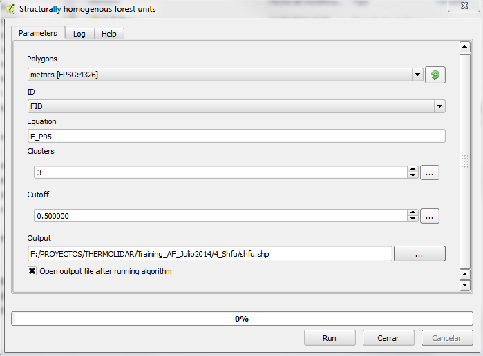
Interface of the “SHFU” module
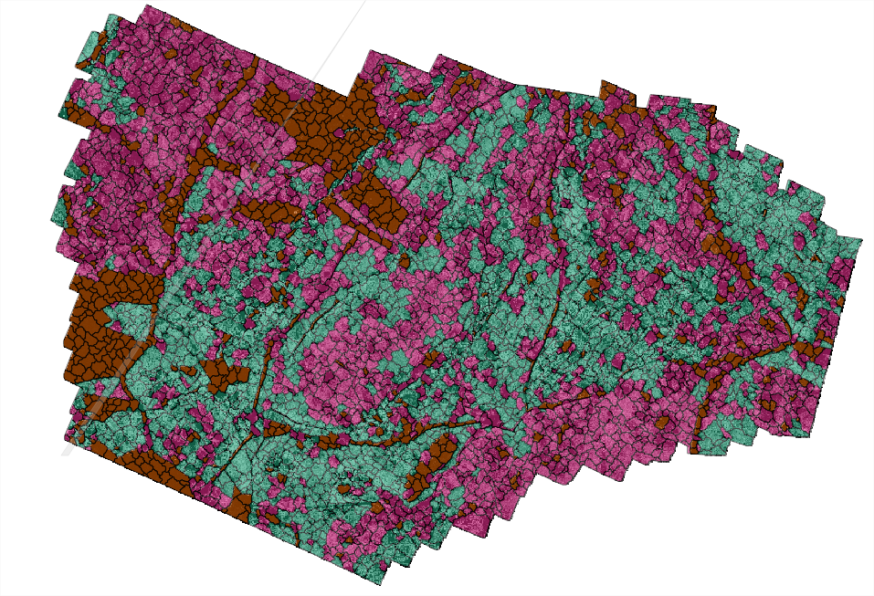
We get as output:
5.2.2.7. Forest Health Classification
5.2.2.8. Unsupervised pixel-based classification
Through this tool raster classify the temperature as many classes as you specify. Temperature classification is performed based on homogeneous units, so many output raster have been defined as SHFU be obtained.
In our case, we obtain three raster classified. Each raster has associated many categories defined temperature.
Interface of the “Unsupervised pixel-based classification” module
We get as output:
5.2.2.9. Unsupervised object-based classification
In the same way that the pixel-oriented, this tool classification raster classify the temperature as many classes as you specify. Temperature classification is performed based on homogeneous units, so many output raster have been defined as SHFU be obtained.
In our case, we obtain three raster classified. Each raster has associated many categories defined temperature.
The difference from the previous tool, is that instead of being classified pixels are classified objects. The classification is made based on the mean value of each of the objects.
Interface of the “Unsupervised object-based classification” module
We get as output: